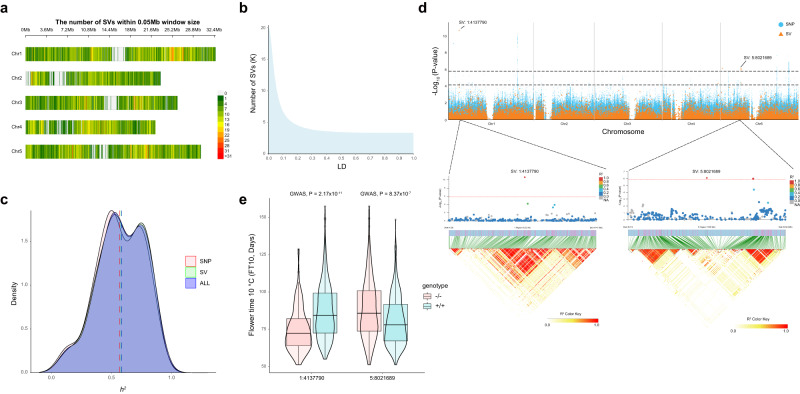
Fig. 6. Contribution of structural variants (SVs) to environmental adaptation.

a Genomic distribution of SV from a population of 1,071 worldwide A. thaliana accessions from the 1001 Genomes Project (https://1001genomes.org/) and two additional ecotypes, Tibet-0 and Yilong-0. b Number of SVs (y-axis) tagged by SNPs at a different linkage disequilibrium (LD) cut-off (x-axis). c Distribution of the proportion of variance (PVE) explained by SNP, SV, and all variants (SV + SNP). d Top: Manhattan plot of SV-GWAS (orange) and SNP-GWAS (blue) for flowering time measured at 10 °C under greenhouse conditions. The dashed black lines are genome-wide significance thresholds for SNP-GWAS (upper, 5.80) and SV-GWAS (lower, 4.17). Middle: Zoomed in genomic regions where SV-GWAS detects unique associations, SV Chr1:4,137,790 and SV Chr5:8,021,689. The diamonds represent the leading variants, and the colors of surrounding variants were highlighted using their LD with corresponding leading variants. Bottom: LD heatmaps of the associated regions. Significance was tested by a standard linear mixed model. e Boxplot illustrating the genotype and phenotype map at two SVs associated with flower time (FT) (SV:1:4137790 -/-: n = 256; +/+: n = 630; SV:5:8021689 -/-: n = 327; +/+: n = 559;) The upper and lower edges of the boxes represent the 75% and 25% quartiles, the central line denotes the median, and the whiskers extend to 1.5× the inter-quartile range (IQR). Significance was tested by a standard linear mixed model. Source data are provided as a Source Data file.