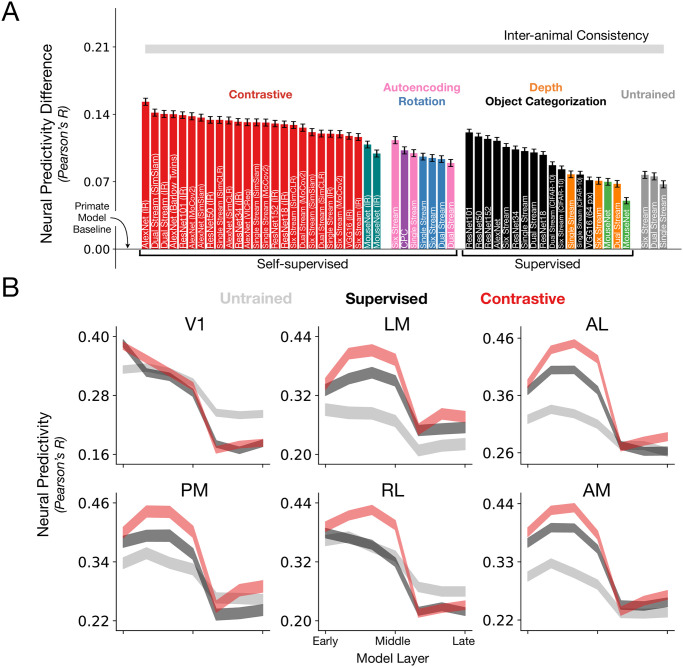
Fig 2. Substantially improving neural response predictivity of models of mouse visual cortex.

A. The median and s.e.m. (across units) neural predictivity difference with the prior-used, primate model of Supervised VGG16 trained on 224 px inputs (“Primate Model Baseline”, used in [14, 15, 36]), under PLS regression, across units in all mouse visual areas (N = 1731 units in total). Absolute neural predictivity (always computed from the model layer that best predicts a given visual area) for each model can be found in Table 2. Our best model is denoted as “AlexNet (IR)” on the far left. “Single Stream”, “Dual Stream”, and “Six Stream” are novel architectures we developed based on the first four layers of AlexNet, but additionally incorporates dense skip connections, known from the feedforward connectivity of the mouse connectome [34, 35], as well as multiple parallel streams (schematized in S1 Fig). CPC denotes contrastive predictive coding [32, 37]. All models, except for the “Primate Model Baseline”, are trained on 64 px inputs. We also note that all the models are trained using ImageNet, except for CPC (purple), Depth Prediction (orange), and the CIFAR-10-labeled black bars. B. Training a model on a contrastive objective improves neural predictivity across all visual areas. For each visual area, the neural predictivity values are plotted across all model layers for an untrained AlexNet, Supervised (ImageNet) AlexNet and Contrastive AlexNet (ImageNet, instance recognition)—the latter’s first four layers form the best model of mouse visual cortex. Shaded regions denote mean and s.e.m. across units.