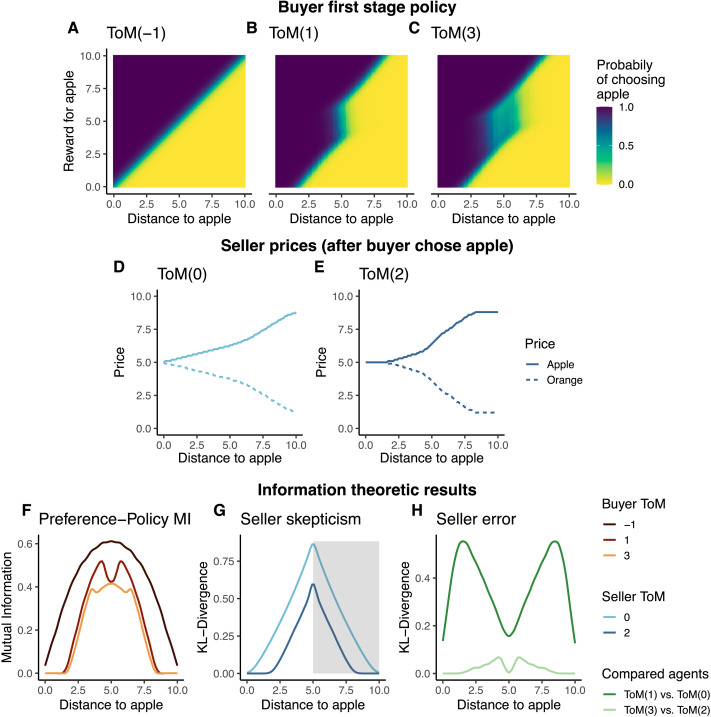
Figure 3. .

(A–C) Buyer policy in first stage as a function of the distance d(apple) and the preference towards the apple, r(apple), shown by different ToM-levels. Here, we are using a soft policy with a temperature of β = 0.5, as for example in equation 6a. The policies are symmetric because of the constraints. Notice the ruse in ToM(1) and ToM(3), who shift their policies. (D–E) Seller prices, m, after a buyer chose the apple as a function of the distance to the apple, d(apple), for the two different seller ToM-levels. ToM(2) discards the evidence at the extremes. (F) Amount of deception by the different ToM buyers quantified by the mutual information between the buyer’s apple preferences and the probability that they will pick an apple. ToM(1) and ToM(3) show lower values, effectively hiding their preferences. (G) Strength of the seller’s belief update quantified by the KL-Divergence between their (flat) prior and posterior over the apple preferences, after observing the buyer choose the closer and thus more likely object (apple in left half, orange in shaded right half). (H) Dissimilarity between the ToM(k) seller’s assumed policy and the ToM(k + 1) buyer’s actual policy, simultaneously showing the hacking success of the buyer and error of the seller.