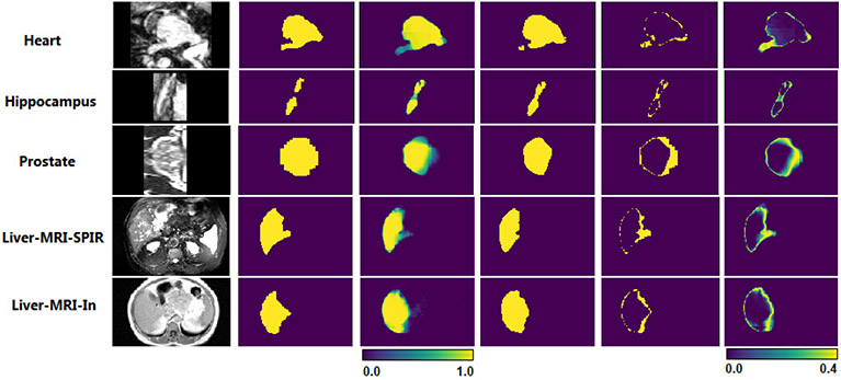
Fig. 3.
Examples prediction uncertainty maps produced by a model trained to segment a heterogeneous pool of datasets. From left, the first column shows a slice of the image. The second column is the ground-truth segmentation map. The third column is the model’s predicted probability map (in the range [0,1]) that each voxel is a foreground voxel. The fourth column is the probability map thresholded at 0.5, showing the binary prediction of the model. The fifth column is the binary difference between the ground-truth (second column) and prediction (fourth column). In other words, the fifth column shows voxels where the model makes wrong predictions. The last column shows a voxel-wise prediction uncertainty map computed as where is the predicted class probability for the voxel (in the range [0, −0.5 log(0.5)]). Note that all images in this figure are in-distribution data.

