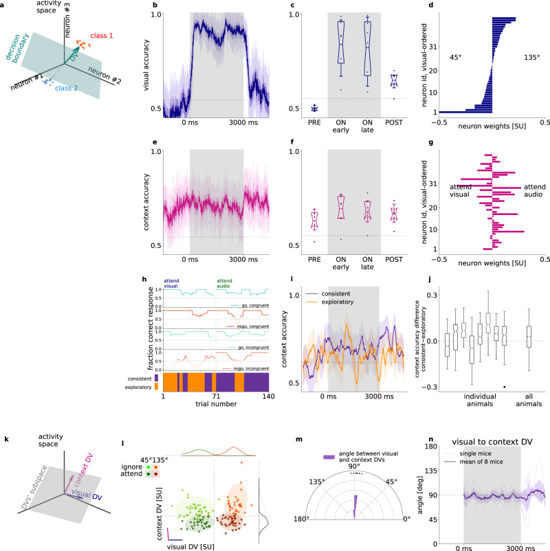
Fig. 3. Representation of task context in population activity.
a Illustration of the decision vector of a linear decoder constructed for neural activity. A linear decoder discovers a decision boundary (green surface) in the activity space which separates responses in individual trials (dots) in two conditions (red and blue). The decision boundary can be uniquely characterized by the decision boundary normal vector (decision vector, DV, green arrow). b Visual decoder performance in 50 ms time windows at 10 ms sliding resolution for an example animal. Gray background represents the stimulus presentation period. Gray dashed line indicates shuffled baseline. Note that firing rates are estimated by using convolution kernels with 100-ms characteristic width and therefore decoders contain information from future time points, resulting in a slight increase in decoder performance prior to stimulus onset. c Average performance of visual decoder for all animals (dots, n = 8), prior to stimulus onset (PRE), during stimulus (ON), and after stimulus (POST). Box and whiskers denote 25–75, and 2.5–97.5 percentiles respectively, midlines are mean, notches are 95% confidence level error of the mean. Gray dashed line indicates shuffled baseline. d Contributions of individual neurons to the visual decoder (decoder weights) arranged according to the magnitude of the weights. e-g same as (b–d) but for decoding context from the population activity. Ordering of neurons on g is the same as that on (d). h Behavioral performance in ‘go’ or ‘no-go’, and congruent or incongruent trials (top four panels) for an example animal. Darker color indicates behavioral performance exceeding chance. Bottom panel: Consistent (purple) and exploratory trials (orange). i Context decoders, as in (e), using only consistent (purple) or exploratory (orange) trials from both contexts; s.e.m. of leave one out mean accuracy (bands), effective chance level (gray dashed line), same animal as (h). j Distribution of time-resolved accuracy difference between consistent and exploratory accuracy, excluding timepoints where both consistent and exploratory accuracies are below chance for individual animals (left), and for all animals concatenated (right); each animal has nT > 450 time points for the distribution, boxplot parameters as in (c). k Combination of multiple DV bases forms a new basis that defines a higher dimensional subspace of task relevant population activity. l Population responses of an example animal, averaged over the first 1.5 s of stimulus presentation projected on the DV subspace in individual trials (dots), and their estimated normal distribution (mean and 2 std, shaded ovals) in different task contexts (dark and light) and with different visual stimuli presented (red and green). Purple and blue lines denote the DV directions of context and visual decoders, respectively. Histograms show population responses projected on orthogonal components of single DVs. m Histogram of the angle between context and visual DVs across animals (dots). n Time course of the angle between the visual and context decoders throughout the trial, distribution of animals (n = 8, gray faint lines) mean (purple thick line) and s.e.m. (faint purple band).

