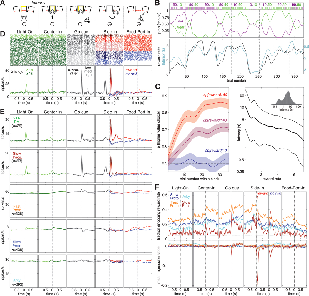
Figure 3. Subpopulation-specific value and RPE coding in the instrumental task.

(A) Schematic of key instrumental task events.

(B) Example behavioral session. The session is divided into blocks of 35–45 trials each (delineated by dashed lines). During each block the reward probabilities for each choice are held constant; these numbers are given at the top of the panel with the reward probability for left and right choices in purple and green, respectively. The higher reward probability is in bold. The ticks below the reward probabilities show each choice made during this session; left choices in purple, right choices in green, long ticks for rewarded trials, short ticks for unrewarded trials. The probability of making each choice (generated from smoothing the individual choices with a Gaussian, 20-trial SD) is plotted below the ticks. Bottom panel, reward rate (black, left Y-axis) is plotted with latency (cyan, right Y-axis). Latency is plotted on an inverted logarithmic scale.

(C) Average rat behavior during instrumental learning sessions (89 sessions in 5 rats). Left, average evolution of choice preference during a block. Blocks are grouped by the difference in reward probability between the two choices—Δp[reward] can be 80 (10:90 or 90:10 blocks, red), 40 (e.g., 90:50, 10:50 blocks, purple), or 0 (e.g., 50:50, 90:90 blocks, blue). The average probability of choosing the higher-reward option is plotted as a function of trial number within the block; shaded areas denote SE. Right, average latency to initiate a trial as a function of current reward rate, plotted on a logarithmic scale. Thick line is median (50th percentile), thin lines show quartiles (25th, 75th percentiles). Inset, histogram of latencies from all sessions (logarithmic bins).

(D) Example of a Slow Pacemaker cell recorded during instrumental learning (same cell as Figure 2D). In the first two panels, raster ticks are colored by latency: spikes fired on “engaged” trials (latency <1 s) are light green, other trials are dark green. In the 3^rd panel (“go cue”), trials are sorted by reward rate and divided into terciles. Low, medium, and high reward rates are denoted by dark, medium, and light gray ticks, respectively. In the 4^th panel (“side in”), trials are divided by reward (red/blue, as in Figure 2D) and reward rate; darker colors denote lower reward rates. For the last panel, trials are just divided by reward delivery; some unrewarded trials are omitted because the rat did not visit the food port. Bottom, same data as above, expressed as a firing rate. In the 4^th panel, all trials within the same reward rate category are averaged together before Side-in, but after side in rewarded and unrewarded trials are averaged separately. See Figures S5, S6 for examples in other cell types.

(E) Activity in the instrumental task averaged across all cells of a given type. The top row shows the activity of VTA dopamine cells (Mohebi et al. 2019) for comparison to GPe cell types (rows 2–5).

(F) Top, fraction of cells whose value (reward rate) regression slope is significantly different from zero as a function of time in trial. All trials are included in the regression model before the “side in” event; after “side in”, rewarded (left) and unrewarded trials (right) are analyzed separately. Only rewarded trials are shown for the “food port” event. Vertical dashed lines mark the time of each event; horizontal dashed line marks the 5% fraction expected by chance. To significantly exceed this chance level (binomial test, p < 0.05), the fraction required depends on the number of cells in the subpopulation, as follows: Fast Protos (n = 338), 6.9%; Slow Protos (n = 438), 6.7%; Arkys (n = 292), 7.0%; Slow Pacemakers (n = 93), 8.5%. See also Figure S3. Bottom, mean regression slope for value for each GPe cell type; shaded areas show SE.