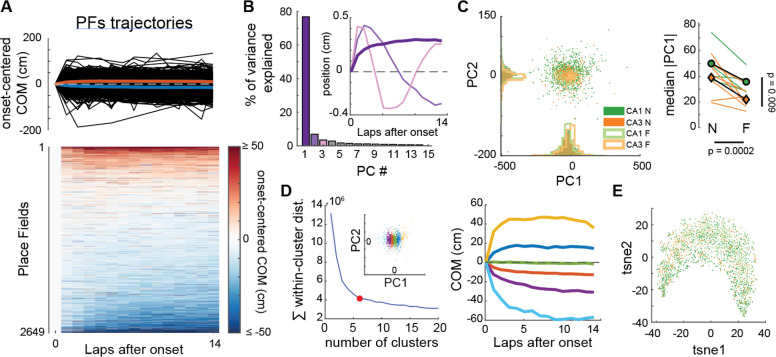
Figure 5. CA1 and CA3 PFs show a continuum of a single type of non-linear trajectory in experimental data.
A. COM trajectories for all PFs recorded in CA1 and CA3 (same data as in Fig. 1). We used linear interpolation to infer the COM position on laps without activity, but results were similar without interpolation. Top: superimposed trajectories (black). Colored curves correspond to averages of PFs with negative (blue) or positive (red) average COM position. Bottom: same data in matrix form, each row being a PF.
B. PCA was performed on the ensemble of trajectories shown in A. The first principal component PC1 explained 76.8% of the variance, revealing a non-linear trajectory template with a large shift during the first few laps (inset, dark purple bold curve — note that the polarity of the trajectory is irrelevant here because projection scores can be positive or negative, see Fig S12B). All other principal components revealed non-linearities but explained little variance each.
C. Left: Scatterplot of the PC1 and PC2 projections of all recorded PFs, color-coded by subfield and familiarity. Right: Animal-wise ANOVA (see Fig. 1D; colored lines are individual mice, symbols are averages). There is a significant effect of both the subfield and familiarity on PC1 scores. Median Absolute PC1 Score ~ 1 + Subfield + Familiarity + (1 + Familiarity | Mice): Subfield: F(1,19) = 8.32, p = 0.0095; Familiarity: F(1,19) = 20.33, p = 0.00024; The interaction was excluded because not significant.
D. Left: K-means clustering of all PFs trajectories using all principal components. Goodness-of-fit was optimal for 6 clusters (red dot = elbow), but clusters simply corresponded to segments of the PC1 scores (inset). Right: The color code is the same as in the left inset. Average COM trajectory for each k-means cluster reveals a continuum of the same PC1-like non-linear trajectory.
E. non-linear dimensionality reduction (tSNE) confirmed the PCA analysis: COM trajectories do not form separate clusters but are spread along a continuum, with CA1N, CA1F, CA3N and CA3F PFs distributed in a salt-and-pepper fashion (color-code as in C).

