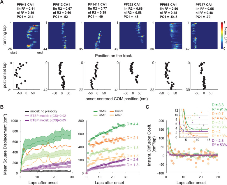
Figure 7. The probability of shift-inducing BTSP-triggering events decays to a constant after PF emergence.

A. Example of PFs showing abrupt shifting late after PF emergence, resulting in zigzag COM trajectories (bottom). PF 1471 (CA1) and 2504 (CA3) in Fig. 6D are other examples with multiple shifting events.

B-C. Diffusion analysis on PFs defined over at least 30 laps.

B. Mean Squared Displacement of the COM (MSD) as a function of post-onset laps (computed over all PFs of each condition: n = 942 for CA1N, 880 for CA1F, 222 for CA3N,100 for CA3F and 500 for each model). For a random walk in a 1D environment such as our linear track, MSD = 2*D*laps, D being the diffusion coefficient. Right: MSD with 95% bootstrapped confidence interval for each condition and model. The large CIs of CA3 were omitted for readability. Left: linear regression on the MSD from lap 4 to lap 30 shows that PF shifting after lap 3 is well explained by a random walk with constant diffusion coefficient D. CA1N: R² = 94.2%, p < 0.0001; CA1F: R² = 80.1% p < 0.0001, CA3N R² = 43.1% p = 0.0002, CA3F R² = 20.1% p = 0.019, BTSP model p(CS) = 0.005: R² = 98.3%, p < 0.0001; BTSP model p(CS) = 0.002: R² = 94.5%, p < 0.0001.

C. Alternative method of estimation of D by fitting the derivative of MSD (data points) to a decaying exponential $\text{p1*exp}(-(\mathrm{x}-1)/\mathrm{p2})+\mathrm{p3}$. The asymptotes (p1 parameter, dashed lines) correspond to D and qualitatively match the values estimated by linear regression in panel C.