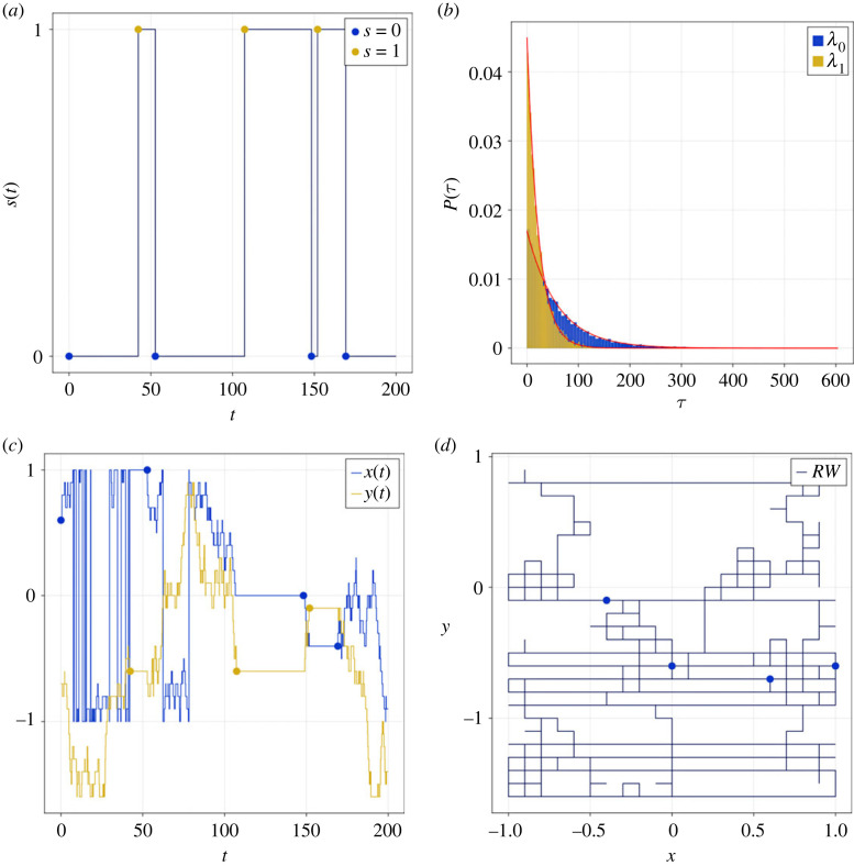
Figure 3.
An example of model dynamics. (a) A realization of the state variable, s(t), is plotted against time. (b) The waiting time distributions for States 0 and 1 are distributed exponentially. Red lines represent theoretical results given by equation (2.4). (c,d) T6SS coordinates are represented as time series (c) and in the xy plane (d). Markers represent transitions between States 0 and 1. See table 2 for parameter values.

