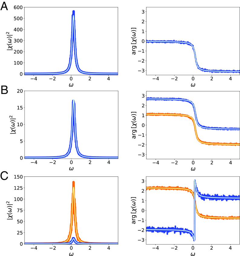
Fig. 4.

Susceptibility functions χ_e(ω) of the variable $Q_1^{*}$ (x(t)) for the different models with the same parameters as in Fig. 2 and different perturbation vectors e as indicated. For each model, we show the squared of the absolute value, |χ_e(ω)|², (Left) showing a Lorentzian profile and its angle arg(χ_e(ω)) (Right). The perturbation vectors are e₁ = (1, 0)^⊤ and e₂ = (0, 1)^⊤. (A) The harmonic oscillator β_ev = −3.87i (blue, computations; cyan, theory); (B) Stuart–Landau model β_e1 = 0.641 − 0.297i (orange, computations; yellow, theory), β_e2 = 0.297 + 0.641i, (blue, computations; cyan, theory); (C) SNIC excitable system β_e1 = 1.38 + 1.3i (orange, computations; yellow, theory), β_e2 = −0.54 + 0.19i (blue, computations; cyan, theory).