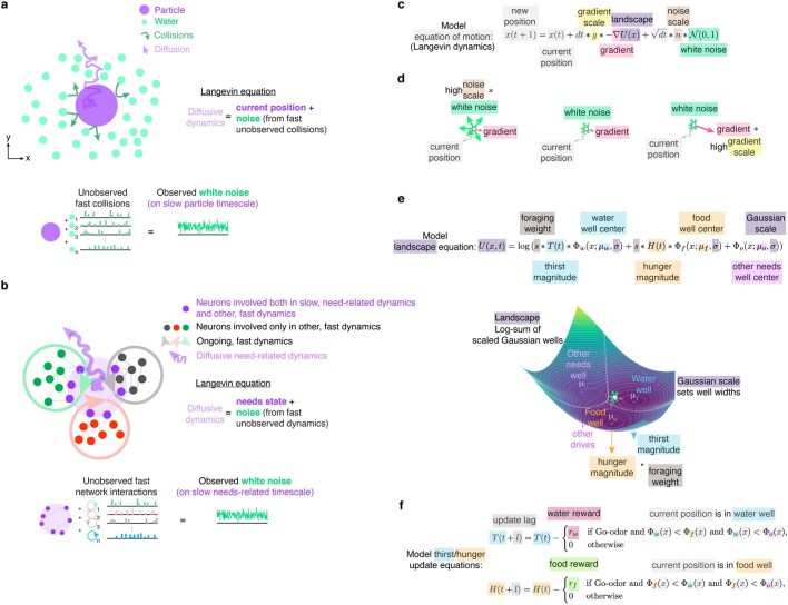
Extended Data Fig. 6. Conceptual similarities between molecular Langevin dynamics and intermixed neural networks.

a, The Langevin equation describes the dynamics of a diffusing particle in water by transforming the unobserved, deterministic, Newtonian dynamics of water molecule collisions (green arrows) with the particle (purple) into a noise contribution to the particle’s position (bottom). This results in a stochastic description of the Brownian motion of the particle (purple arrow). A key feature of this formalism in the study of complex phenomena is the separation of unobserved fast-timescale dynamics (for example, the motion of water molecules) from the observed slow-timescale dynamics of the much larger particle. b, Conceptual application of the Langevin formalism to intermixed neural networks with fast and slow dynamics. Neurons involved in a distributed network with slow-timescale (for example, need-related) dynamics (purple dots) are embedded via mixed functional selectivity into additional networks of neurons (black, red, green dots) with ongoing, unobserved fast-timescale dynamics (gray, pink, light green cycles). By analogy to the Langevin picture of molecular dynamics, the activities of networks with disparate fast time-scale dynamics collide within individual mixed-selective need-related neurons to produce a stochastic noise influence on the slow-timescale dynamics of the need-related network of neurons (bottom), yielding observable diffusive goal dynamics. c, Equation of motion for the forward stimulation of the resolution of needs, following Langevin dynamics. $x\left(t\right)$, position of neural activity across the needs subspace at time $t$. $U\left(x\right)$, the energy landscape function. The new position is the current position plus a small differential contribution by the landscape gradient (scaled by the gradient scale $g$) and Gaussian white noise (scaled by the noise scale $n$). $\mathit{dt}$, the discretized time step. d, Graphical depiction of how the $n$ and $g$ terms contribute to the dynamics. Left, high noise scale $n$ relative to gradient scale $g$ results in noise-dominated dynamics. Middle, balanced scales and dynamics. Right, low noise scale $n$ relative to gradient scale $g$ results in dynamics dominated by the landscape shape. e, Equation for the shape of the time-varying needs landscape $U(x,\mathit{t})$. The landscape consists of a log-sum of scaled Gaussian wells. Gaussian wells, $\mathrm{\Phi }\left(x\right)$, are defined as the negative of the multivariate probability density function. For simplicity, well centers ${\mu }_w$,${\mu }_f$, and ${\mu }_o$ corresponding to the wells for water, food, and other needs are set on an equilateral triangle, and the Gaussian scale parameter controlling the Gaussian widths are set to a common parameter $\sigma$. The water and food well depths are scaled by the time-varying thirst magnitude $T\left(t\right)$ and hunger magnitude $H\left(t\right)$, respectively, as well as by a “foraging” scale factor $s$ that linearly relates the experimental normalized need measurements to the model need magnitude values. f, $U(x,\mathit{t})$ changes across time through changes in thirst and hunger magnitudes. Thirst and hunger magnitudes are decremented after a fixed delay $\mathit{l}$ by factors $r_w$ and $r_f$ upon respective water or food reward collection; reward choices are determined upon Go-cue at time $\mathit{t\text{'}}$ by the location $x\left(\mathit{t\text{'}}\right)$ within a fixed segmentation of the need space into food, water, or other zones. See Methods for full implementation details.