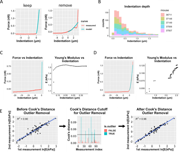
Figure 2: Data filtering process, including Cook’s distance for outlier removal.

A) Representative force-indentation plots (red) illustrating curve fitting quality, with the Hertz model fit shown in blue. The “good” fit (left) demonstrates a reliable curve fit that would be retained for further analysis, while the “poor” fit (right) exhibits inadequate fitting and would be excluded from the analysis. B) Histogram of sample indentation depths. Each color represents data from one animal. Most measurements did not exceed a 1 μm indentation depth, and any measurements with an indentation depth greater than 2 μm were removed from the analysis. C) Fitted Young’s modulus values vs. indentation depth at which the force-indentation curve was truncated for analysis purposes. The plot on the left shows a sample force-indentation plot for an indentation depth < 2 μm, and the plot on the right shows the fitted Young’s modulus (E) values as a function of indentation depth for that force-indentation measurement. D) Similar plots are shown for a measurement from the same animal where the indentation depth exceeded 2 μm. The Young’s modulus values show much more variability and a strong dependence on the indentation depth. E) Overview of the use of Cook’s distance outlier removal. Log-transformed Young’s modulus estimates from the first and second measurements at the same location for one eye are plotted against each other and linearly regressed (left plot). Cook’s distance is used to determine outliers (middle plot, shown in blue), indicating discordance between repeated measurements at the same point, and the regression is re-plotted without outliers (right plot). This process was applied to data from each eye.