TWO-SAMPLE TESTS FOR MULTIVARIATE REPEATED MEASUREMENTS OF HISTOGRAM OBJECTS WITH APPLICATIONS TO WEARABLE DEVICE DATA

Abstract

Repeated observations have become increasingly common in biomedical research and longitudinal studies. For instance, wearable sensor devices are deployed to continuously track physiological and biological signals from each individual over multiple days. It remains of great interest to appropriately evaluate how the daily distribution of biosignals might differ across disease groups and demographics. Hence, these data could be formulated as multivariate complex object data, such as probability densities, histograms, and observations on a tree. Traditional statistical methods would often fail to apply, as they are sampled from an arbitrary non-Euclidean metric space. In this paper we propose novel, nonparametric, graph-based two-sample tests for object data with the same structure of repeated measures. We treat the repeatedly measured object data as multivariate object data, which requires the same number of repeated observations per individual but eliminates any assumptions on the errors of the repeated observations. A set of test statistics are proposed to capture various possible alternatives. We derive their asymptotic null distributions under the permutation null. These tests exhibit substantial power improvements over the existing methods while controlling the type I errors under finite samples as shown through simulation studies. The proposed tests are demonstrated to provide additional insights on the location, inter- and intra-individual variability of the daily physical activity distributions in a sample of studies for mood disorders.

1. Introduction.

Repeated measures are frequently obtained to capture the within-individual variation and enhance the data reproducibility. For example, studies using accelerometers that examine physical activities (PA) often observe individuals’ 24-hour activity profiles repeatedly over several days or weeks (Burton et al. (2013), Crescenzo et al. (2017), Krane-Gartiser et al. (2014)). Within each day the physical accelerations during movement are recorded with a high frequency and processed into a time series of activity intensity metrics, such as activity counts, vector of magnitude (VM), or Euclidean norm minus one (ENMO) over certain epoch lengths (e.g., five, 15 or 60 seconds). Commonly extracted markers from accelerometry data include the total amount of PA such as total log activity intensities and step counts (Varma et al. (2018)) and time spent in different activity intensity levels. In particular, proportion of time spent in sedentary behavior (SB), light (LPA), and moderate-to-vigorous physical activity (MVPA) have been reported to meaningfully correlate with physical and mental functioning and health (Crescenzo et al. (2017), Faurholt-Jepsen et al. (2012), Murray et al. (2020)). However, there remain several known limitations in these traditional PA endpoints. First, metrics such as time spent in SB, LPA and MVPA reduce the continuous activity profiles into a composition of only three discrete categories, resulting in a great loss of the rich information captured by the densely measured raw accelerometry data. In fact, MVPA might be relatively sparse in a largely sedentary population and are less sensitive to meaningful clinical differences within the population. Second, these variables are determined with a priori selected cutpoints. Yet there is a lack of consensus of cutpoints for data collected across study populations (e.g., children vs. adults, diseased vs. healthy individuals), type of devices, and wearing positions (e.g., hip vs. wrist) (Leeger-Aschmann et al. (2019), Schrack et al. (2016)). It has also been reported that the recording frequency, the choice of epoch length, and wear-time algorithms during processing steps could significantly vary the endpoints and potentially lead to inconsistent conclusions (Banda et al. (2016)). Hence, it remains challenging to compare findings across studies with these traditionally derived metrics.

Instead of relying upon a few discrete categories, defined by relatively arbitrary cutpoints, recently increasing attentions have been paid to modeling the continuous distribution of the raw daily activity intensities (Keadle et al. (2014), Schrack et al. (2016), Yang et al. (2020)). In this paper we also take the daily activity histogram for each individual as the observed outcome and develop statistical methods that compare density objects between groups. As an illustration, we plotted the observed activity data from one individual over four days (two weekdays and two weekends) in Figure 1 from the National Institute of Mental Health (NIMH) Family Study of Spectrum Disorders (Merikangas et al. (2014, 2019)). Their time-specific activity intensities at one-minute intervals are shown on the top row, and the corresponding histograms of activity intensities in log-transformed scale are shown on the bottom. As Figure 1 shows, despite the overall similarity in the time-specific activity patterns across days, the evident shifts in schedules from weekdays to weekends might not be of biological interests. Hence, a second advantage of directly modeling the daily activity distributions is that it avoids the need for registering time stamps across days (Wrobel et al. (2019)).

Fig. 1.

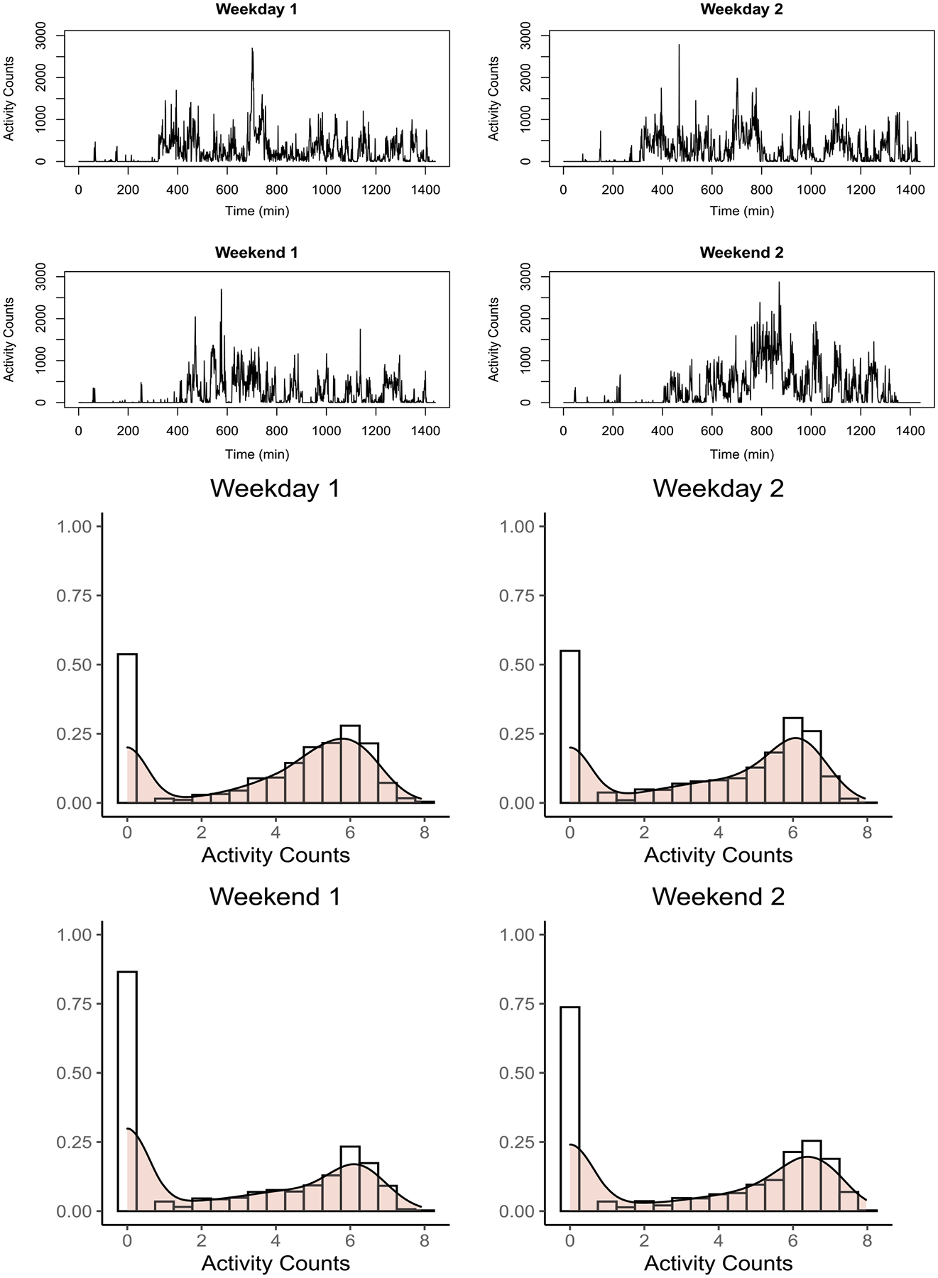
Activity intensities for a randomly chosen individual over four days. Top: Trends of activity intensities; bottom: histograms and densities of activity intensities.

We consider the problem of testing whether the activity density functions or distributions are significantly different between individuals from various clinical groups. As previously noted, the conventional representations of time spent in different levels of PA are derived from discretized distributions using predetermined cutpoints. To minimize the loss of information, we will be working with the entire probability densities of the continuous daily activity intensities. Our challenges are twofold. First, probability densities, as characterized by the histograms of the daily physical activity intensities, are non-Euclidean, and hence many traditional two-sample test statistics are no longer applicable. Second, physical activity tracking over multiple days results in repeated probability densities. As far as we know, there are few existing methods that could handle within-individual dependency in the complex object data.

While two-sample testing for mutivariate objects in Euclidean space or even infinite dimensional space has been studied extensively in the statistics’ literature, fewer tools are available for two-sample testing when the data are samples of density or distributional functions. To deal with a wide range of data types, nonparametric tests are preferable. Friedman and Rafsky (1979) proposed the first practical test as an extension of the Wald–Wolfowitz runs test to multivariate data. This framework has been extended to other graph-based testing methods. For example, Rosenbaum (2005) used the minimum distance pairing (MDP); Schilling (1986) and Henze (1988) adopted the nearest neighbor graph (NNG); Chen and Friedman (2017) and Chen, Chen and Su (2018) proposed a generalized edge-count test and a weighted edge-count test to address the problems under scale alternatives and unequal sample sizes, respectively. Recently, an extension of analysis of variance for metric space valued data objects was proposed by Dubey and Müller (2019), where Fréchet mean and variance are used to construct the test statistic. Yang et al. (2020) proposed quantlets as basis functions to approximate the quantile function objects in a regression setting.

However, most of these existing tests for object data assume that the observations are independent which cannot be directly applied to repeated measures of object data where within-individual observations are correlated. One simple way to deal with this issue is to apply these tests to the average of the within-individual measures and convert the problem into a standard two-sample test for independent object observations (Dawson and Lagakos (1993)). However, it is not trivial to define the average of non-Euclidean object data. In addition, taking averages oversimplifies the true complexity of data and ignores the within-individual variability that could also be clinically relevant when studying individuals’ behaviors and mood (Murray et al. (2020)).

We propose a new nonparametric testing framework for density data with repeated measures. This framework builds upon graph-based two-sample testing methods that are flexible and require few assumptions (Chen, Chen and Su (2018), Chen and Friedman (2017)). In particular, to take into account the repeated nature of the data, we consider the between-individual and within-individual similarity graphs defined via the Wasserstein distances between two density functions. Based on the constructed graph, we define several test statistics that are powerful for various possible alternatives, including difference in population Fréchet means, Fréchet variances, and Fréchet covariance. A new permutation null distribution is considered using the between-individual and within-individual similarity graphs. We also derive the asymptotic null distributions of these statistics under the permutation null, facilitating their applications to large data sets.

We evaluate the proposed test statistics using simulations and compare the power with several competing tests developed for density data. Our approaches are used in an extensive analysis to evaluate the effects of age, body mass index, and types of mood disorders on daily activities in the NIMH family study population.

2. Nonparametric tests for density functions with repeated measures based on a similarity graph.

2.1. A permutation null distribution for density data with repeated measures.

To analyze the repeated measurements of activity data, we treat the observed activity densities over $l$ days from each individual as a vector of outcome. We assume that individuals are divided into two groups with ${𝒳}_1,\dots ,{𝒳}_{n_1}$ representing density objects for $n_1$ individuals from group 1 and ${𝒴}_1,\dots ,{𝒴}_{n_2}$ representing densities for $n_2$ individuals from group 2. For a given individual $u$ from group 1, we have ${𝒳}_u=\left(X_{u1},\dots ,X_{ul}\right)$ representing each of the $l$ days’ activity densities. Similarly, for individual $v$ from group 2, ${𝒴}_v=\left(Y_{v1},\dots ,Y_{vl}\right)$.

We assume that each individual density $X_{ui}$ and $Y_{vj}\left(u=\mathrm{1,2},\dots ,n_1;v=\mathrm{1,2},\dots ,n_2\right.;i,j=\mathrm{1,2},\dots ,l)$ belongs to space $𝒟$, where $𝒟$ represents a class of one-dimensional densities such that ${\int }_R{u}^{2}f\left(u\right)\text{d}u<\infty$ for $f\in 𝒟$. For any two random densities $\mathbf{X},\mathbf{Y}\in 𝒟$, we define $d_W$ to be the Wasserstein metric as

$$d_W^2(\mathbf{X},\mathbf{Y})={\int }_R\left\{T\right(u)-u{\}}^2\mathbf{X}(u)\text{d}u,$$

where $T=F_{\mathbf{Y}}^{-1}\circ F_{\mathbf{X}}$ is the optimal transport, and $F_{\mathbf{X}}$ and $F_{\mathbf{Y}}$ are the distribution functions of $\mathbf{X}$ and $\mathbf{Y}$, respectively.

We further assume that $X_{ui}$ and $X_{uj}$ have identical distribution function $F_1$ but might be correlated; similarly, $Y_{vi}$ and $Y_{vj}$ have the same distribution $F_2$. The vector of $l$-day densities ${𝒳}_u,u=1,\dots ,n_1$, however, are independently and identically distributed across individuals according to ${\tilde{P}}_1.{𝒴}_v,v=1,\dots ,n_2$, are i.i.d. according to ${\tilde{P}}_2$.

For a random density $\mathbf{X}\in 𝒟$ from group 1, we define the corresponding group-level Fréchet mean ${\mu }_{F_1}$ and Fréchet variance $V_{F_1}$ as

$${\mu }_{F_1}=\underset{x\in 𝒟}{\text{arg}\text{min }}E\left\{d_W^2(x,\mathbf{X})\right\},V_{F_1}=E\left\{d_W^2\left({\mu }_{F_1},\mathbf{X}\right)\right\}.$$

Similarly, ${\mu }_{F_2}$ and $V_{F_2}$ represent the Fréchet mean and Fréchet variance for a random density $\mathbf{Y}$ from group 2. Given a vector of random densities whose elements are dependent with each other, we define their Wasserstein covariance following the framework in Petersen and Müller (2019). Specifically, for two random densities ${\mathbf{X}}_i$ and ${\mathbf{X}}_j$ from group 1, the Wasserstein covariance is defined as

$${\text{Cov}}_{F_1,ij}=E\left[{\int }_0^1\left\{F_{X_i}^{-1}\left(u\right)-F_{{\mu }_{F_1}}^{-1}\left(u\right)\right\}\left\{F_{X_j}^{-1}\left(u\right)-F_{{\mu }_{F_1}}^{-1}\left(u\right)\right\}\text{d}u\right]$$

where $F_{{\mu }_{F_1}}$ denotes the distribution function of ${\mu }_{F_1}$. Similarly, ${\text{Cov}}_{F_2,ij}$ denotes the Wasserstein covariance between ${\mathbf{Y}}_i$ and ${\mathbf{Y}}_j$ from group 2.

We are interested in testing the null hypothesis $H_0:{\tilde{P}}_1={\tilde{P}}_2$ which implies that the $N=n_1+n_2$ samples are from the same distribution. Based on our motivating examples, group differences in physical activity distributions could occur in mean ${\mu }_{F_1}\ne {\mu }_{F_2}$, between-individual variability $V_{F_1}\ne V_{F_2}$, or within-individual variability among repeated observations ${\text{Cov}}_{F_1,ij}\ne {\text{Cov}}_{F_2,ij}$ for, at least, one $(i,j),i\ne j$ pair. For a given test, any of such alternatives should lead to rejection of the null when the sample sizes are large enough. Instead of imposing any parametric assumptions, we propose a set of nonparametric test statistics based on a similarity graph constructed using pairwise Wasserstein distance, as detailed in Section 2.2 and a permutation procedure to capture these various possible alternatives. The permutation procedure treats the repeated measures from the same individual as the permutation unit. Specifically, the permutation is done by randomly assigning $n_1$ individuals out of the total $N$ individuals to group 1 and the rest to group 2. If an individual is assigned to group 1, then the repeated measures of the individual are labeled as observations from group 1. Note that we do not require equal correlation or exchangeability within individual among repeated observations since our data are observed sequentially over time. However, to ensure the exchangeability across individuals under the null $H_0$, we do require that the number of repeated observations is the same for all the individuals. In the following, when there is no further specification, we use $\mathbf{P},\mathbf{E}$, Var, and Cov to denote probability, expectation, variance, and covariance, respectively, under this permutation null distribution. An illustration of the data structure and distribution assumptions are presented in Figure 3.

Fig. 3.

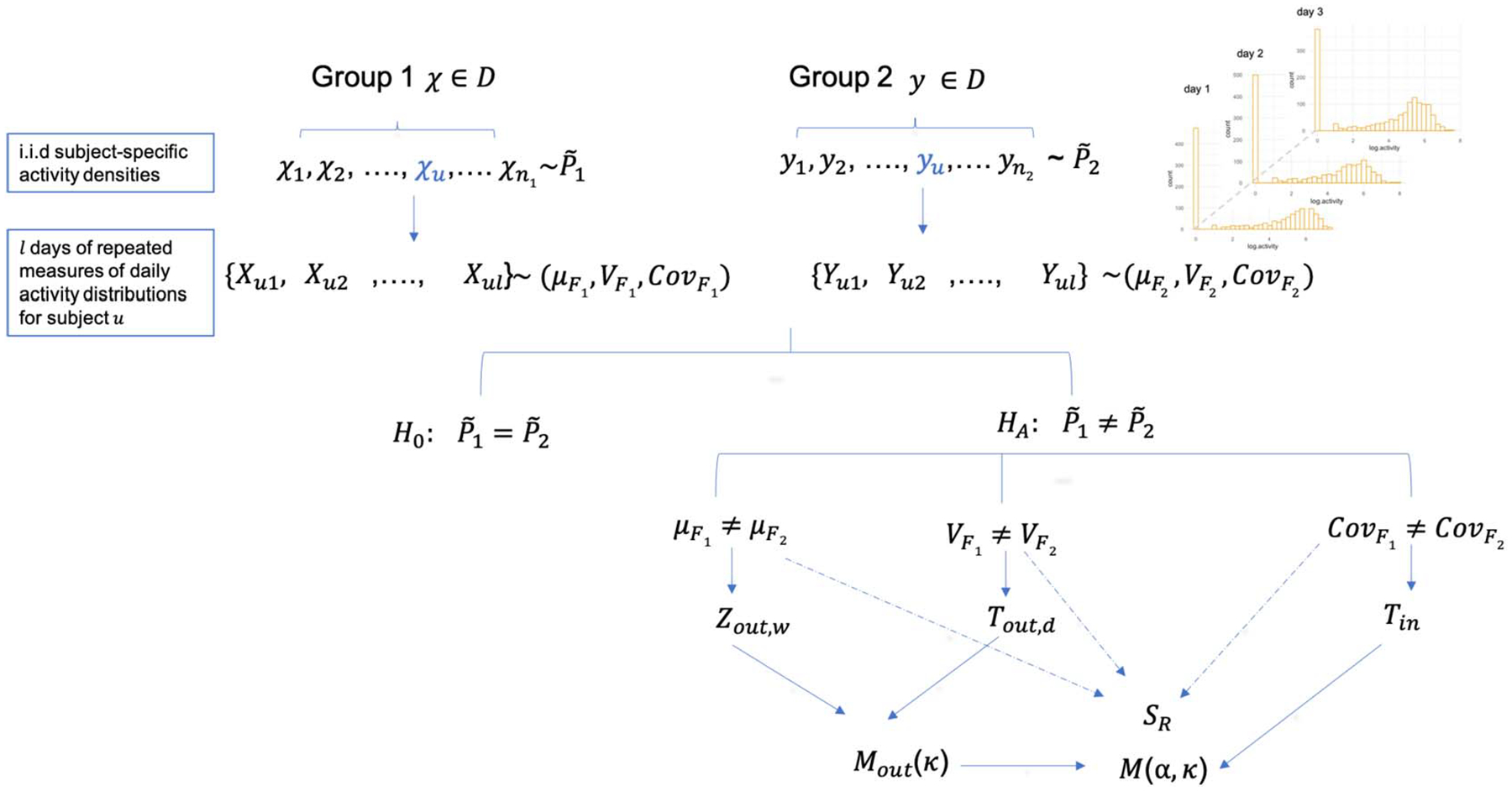
An overview of the repeated data structure, the null hypothesis and various alternatives that each of the proposed test statistics are most suitable for.

2.2. Graph-based statistics for data with repeated measures.

Our proposed test statistics are constructed from a similarity graph that includes both a within-individual graph and a between-individual graph in order to take into account repeated measures. To construct the graph based on the Wasserstein distance $d_W$, we pool all repeated measures from a total of $N=n_1+n_2$ individuals, and construct a similarity graph $G$ as a minimum spanning tree (MST). An MST is a spanning tree that connects all observations that minimizes the sum of the total distances of the edges in the tree. In particular, a $k$-MST is the union of the 1st MST, …, $k$th MST, where the 1 st MST is the MST and the $j$th $(j>1)$ MST is a spanning tree connecting all observations that minimizes the sum of distances across edges under the constraint that this spanning tree does not contain any edge from the previous 1st MST, …, and $(j-1)$th MST. Since the graph-based statistics are usually more powerful under a slightly denser graph (Friedman and Rafsky (1979)), we choose 9-MST for our similarity graph $G$ in our simulation studies and real application, following the recommendation by Chen, Chen and Su (2018). Based on the similarity graph $G$ of all the observations, we further divide its edges into two parts. If an edge connects two observations from the same individual, it belongs to the within-individual similarity graph $G_{\text{in}}$, otherwise, it belongs to the between-individual similarity graph $G_{\text{out}}$ (see Figure 2 for an illustration).

Fig. 2.

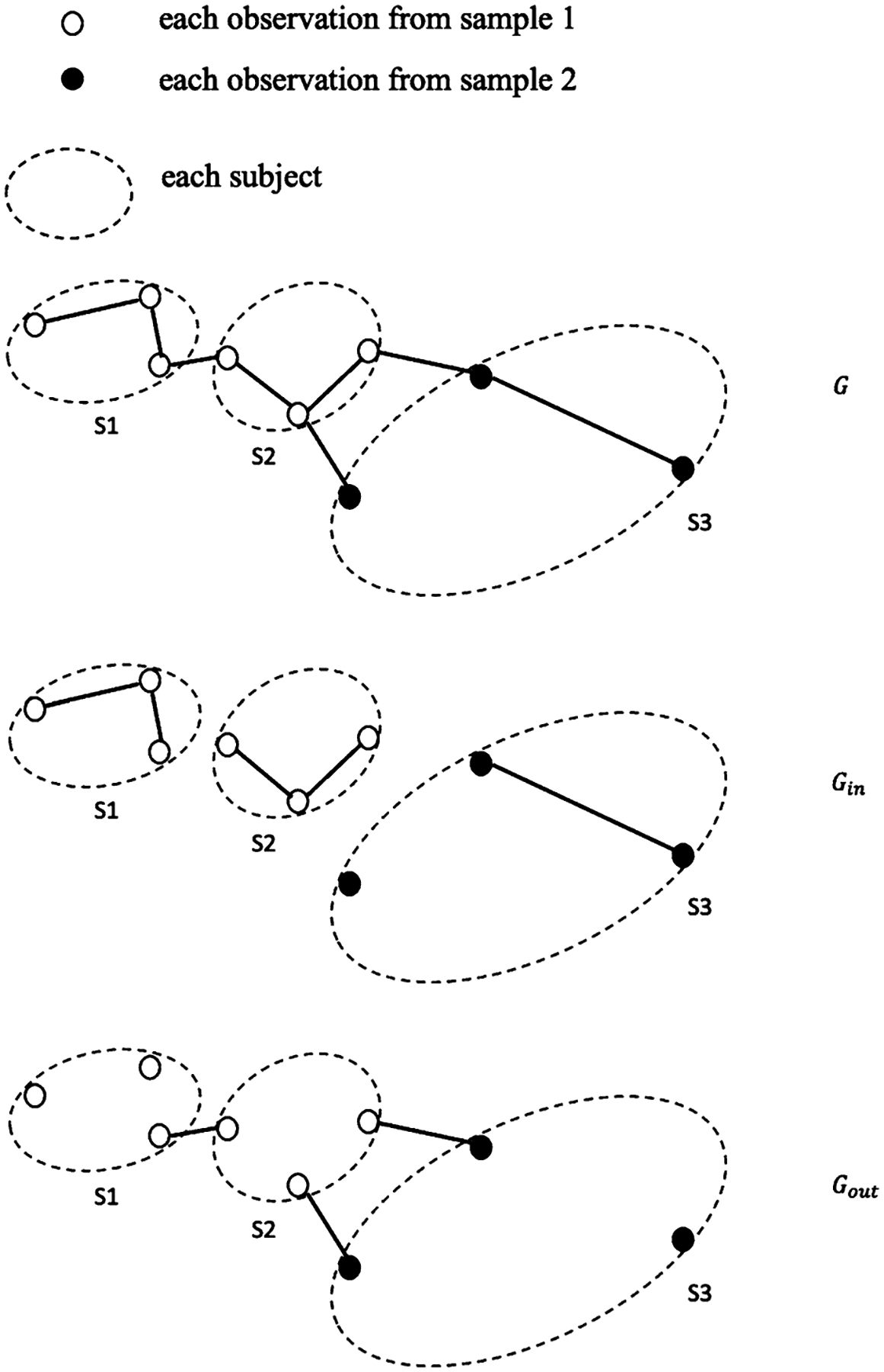
An example of similarity graph $G$, within-individual gragh $G_{\text{in}}$, and between-individual graph $G_{\text{out}}$ for three individuals with repeated measures.

Given a constructed graph $G$, we let $D={\left(D_{uv}\right)}_{N\times N}$ be a symmetric matrix, where $D_{uv}$ denotes the number of edges between individuals $u$ and $v$ in $G$ and let $D_u={\sum }_{v\ne u}{D}_{uv}$ be the total number of edges connecting individual $u$ and others. The total number of edges in $G$ is denoted by $\left|G\right|$. Furthermore, let $g_i$ be an indicator function that takes value 1 when node $i$ belongs to an individual from group 1, and 2 otherwise. We denote an edge in $G$ by the indices of the nodes that are connected by the edge, such as $e=(u,v)$. Define

$$R_{\text{out},k}=\sum _{(i,j)\in G_{\text{out}}}I\left(g_i=g_j=k\right),R_{\text{in},1}=\sum _{(i,j)\in G_{\text{in}}}I\left(g_i=g_j=1\right).$$

Here, $R_{\text{out},k}$ is the number of between-individual edges in $G_{\text{out}}$ that connect observations belonging to the same group $k,k=\mathrm{1,2}.R_{\text{in,}1}$ is the number of within-individual edges in $G_{\text{in}}$ from group 1.

To accommodate various alternatives to the null hypothesis, we consider six different test statistics presented in Table 1. The six test statistics are defined based on different functions of $R_{\text{out},1},R_{\text{out},2}$, and $R_{\text{in,}1}$ and their expectations and variances calculated under the permutation null. These different test statistics are developed for testing the same null $H_0:{\tilde{P}}_1={\tilde{P}}_2$, but their statistical power depends on specific alternatives, as summarized in Figure 3. For each of the test statistics, under $H_0$ and a fixed graph $G$, one could randomly shuffle the group assignments for all individuals to estimate their corresponding null distributions.

Table 1.

Proposed test statistics for the difference of two population distributions of the density functions

Within-individual test

Wasserstein covariance difference

$T_{\text{in}}=\left|Z_{\text{in}}\right|,Z_{\text{in}}=\frac{R_{\text{in},1}-E\left(R_{\text{in},1}\right)}{\sqrt{Var\left(R_{\text{in},1}\right)}}.$

Between-individual test

Mean difference

$Z_{\text{out},w}=\frac{\left(n_2-1\right)R_{\text{out},1}+\left(n_1-1\right)R_{\text{out},2}-E\left(\left(n_2-1\right)R_{\text{out},1}+\left(n_1-1\right)R_{\text{out},2}\right)}{\sqrt{Var\left(\left(n_2-1\right)R_{\text{out},1}+\left(n_1-1\right)R_{\text{out},2}\right)}}.$

Variance difference

$T_{\text{out},d}=\left|Z_{\text{out},d}\right|,Z_{\text{out},d}=\frac{R_{\text{out},1}-R_{\text{out},2}-E\left(R_{\text{out},1}-R_{\text{out},2}\right)}{\sqrt{Var\left(R_{\text{out},1}-R_{\text{out},2}\right)}}.$

Overall difference

$M_{\text{out}}(\kappa )=\text{max}\left\{T_{\text{out},d},\kappa Z_{\text{out},w}\right\}.$

Joint between and within-individual test

Sum-type test

$S_R={\left(\begin{array}{c}{R}_{\text{out},1}-E\left(R_{\text{out},1}\right)\\ R_{\text{out},2}-E\left(R_{\text{out},2}\right)\\ R_{\text{in},1}-E\left(R_{\text{in},1}\right)\end{array}\right)}^T{\Sigma }^{-1}\left(\begin{array}{c}{R}_{\text{out},1}-E\left(R_{\text{out},1}\right)\\ R_{\text{out},2}-E\left(R_{\text{out},2}\right)\\ R_{\text{in},1}-E\left(R_{\text{in},1}\right)\end{array}\right),$ where $\Sigma =Var\left({\left(R_{\text{out},1},R_{\text{out},2},R_{\text{in},1}\right)}^T\right)$.

Max-type test

$M(\alpha ,\kappa )=\text{max}\left\{T_{\text{in}},\alpha M_{\text{out}}(\kappa )\right\}.$

Specifically, $T_{\text{in}}$ builds upon the contrast of within-individual edge counts between group 1 and group 2, holding the total number of edge counts to be constant. Hence, it captures the covariance among the repeatedly observed densities. Rejecting $H_0$, based on $T_{\text{in}}$, implies that ${\text{Cov}}_{F_1}\ne {\text{Cov}}_{F_2}$, suggesting that the group difference occurs in the amount of day-to-day variability in daily activity distributions.

The next three test statistics $Z_{\text{out},w},T_{\text{out},d}$, and $M_{\text{out}}\left(\kappa \right)$ are developed to capture the group difference in the marginal distribution of individual activity densities $F_1$ and $F_2$. In particular, $Z_{\text{out},w}$ evaluates the mean difference between the two groups, and rejecting $H_0$ implies that ${\mu }_{F_1}\ne {\mu }_{F_2}$. Similarly, $T_{\text{out},d}$ examines the group difference in between-individual variances and rejects $H_0$ when $V_{F_1}\ne V_{F_2}$. Finally, $M_{\text{out}}\left(\kappa \right)$ combines the comparison in both mean and variance by taking the maximum of the two. Note that these statistics are adapted from the existing formulations from Zhang and Chen (2022). However, this is not a direct application from the previous work due to the existence of repeated observations per individual. Our novelty lies in expanding the similarity graph to include both $G_{\text{out}}$ and $G_{\text{in}}$ that allow more than one edge connecting between any pair of individuals. Since the edges in $G_{\text{out}}$ are correlated with those in $G_{\text{in}}$, new derivations are needed to obtain the asymptotic distributions. The two final statistics $S_R$ and $M(\alpha ,\kappa )$ combine the previously defined statistics in a weighted fashion and flexibly capture differences occurred in both the between-individual distributions $F_1$ and $F_2$ as well as the within-individual covariance.

2.3. Analytic expressions of the new statistics.

In the following we first derive the exact analytic expressions for the expectation and variance of $\left(R_{\text{out},1},R_{\text{out},2},R_{\text{in},1}\right)$ so that the proposed test statistics in Section 2.2 can be computed efficiently. The analytic expressions are provided in the following theorem. The detailed proof could be found in the Supplementary Material (Zhang et al. (2022)).

Theorem 2.1. Under the permutation null, the analytic expressions of the expectation of ${\left(R_{\text{out},k},R_{\text{in},1}\right)}^T,k=\mathrm{1,2}$ are

$$\mathbf{E}\left(R_{\text{out,}k}\right)=\left|G_{\text{out }}\right|\frac{n_k\left(n_k-1\right)}{N(N-1)},\mathbf{E}\left(R_{\text{in,}1}\right)=\left|G_{\text{in}}\right|\frac{n_1}{N}.$$

The analytic expressions of the variances are

$$\begin{gathered} \mathbf{\text{Var}}\left(R_{\text{out},k}\right)=\frac{n_1{n}_2\left(n_1-1\right)\left(n_2-1\right)}{N\left(N-1\right)\left(N-2\right)\left(N-3\right)}\times \left\{\frac{1}{2}\sum _{u\ne v}{D}_{uv}^2+\frac{n_k-2}{N-n_k-1}\left(\sum _u{D}_u^2-\frac{4{\left|G_{\text{out}}\right|}^2}{N}\right)-\frac{2}{N\left(N-1\right)}{\left|G_{\text{out}}\right|}^2\right\}, \\ \mathbf{\text{Var}}\left(R_{\text{in},1}\right)=\frac{n_1{n}_2}{N(N-1)}\left(\sum _u{D}_{uu}^2-\frac{{\left|G_{\text{in}}\right|}^2}{N}\right), \end{gathered}$$

and the analytic expressions of covariance are

$$\begin{gathered} \mathbf{\text{Cov}}\left(R_{\text{out,}1}{R}_{\text{out,}2}\right)=\frac{n_1{n}_2\left(n_1-1\right)\left(n_2-1\right)}{N\left(N-1\right)\left(N-2\right)\left(N-3\right)}\times \left\{\frac{1}{2}\sum _{u\ne v}{D}_{uv}^2-\left(\sum _u{D}_u^2-\frac{4}{N}{\left|G_{\text{out }}\right|}^2\right)-\frac{2}{N\left(N-1\right)}{\left|G_{\text{out}}\right|}^2\right\}, \\ \mathbf{\text{Cov}}\left(R_{\text{out,}k}{R}_{\text{in},1}\right)=(-1{)}^{k+1}\frac{n_1{n}_2\left(n_k-1\right)}{N(N-1)(N-2)}\left(\sum _{u=1}^N{D}_{uu}{D}_u-\frac{2}{N}\left|G_{\text{in}}\right|\left|G_{\text{out}}\right|\right). \end{gathered}$$

Using the results of Theorem 2.1, we can check that, under the permutation null, $\mathbf{E}\left(Z_{\text{out,}w}\right)=\mathbf{E}\left(Z_{\text{out,}d}\right)=\mathbf{E}\left(Z_{\text{in}}\right)=0,\mathbf{V}\mathbf{a}\mathbf{r}\left(Z_{\text{out,}w}\right)=\mathbf{V}\mathbf{a}\mathbf{r}\left(Z_{\text{out,}d}\right)=\mathbf{V}\mathbf{a}\mathbf{r}\left(Z_{\text{in}}\right)=1$, and $\mathbf{C}\mathbf{o}\mathbf{v}\left(Z_{\text{out,}w},Z_{\text{out,}d}\right)=0,\mathbf{C}\mathbf{o}\mathbf{v}\left(Z_{\text{out,}w},Z_{\text{in}}\right)=0$. In addition,

$$\mathbf{\text{Cov}}\left(Z_{\text{out,}d},Z_{\text{in}}\right)=\frac{\sum _{u=1}^N{D}_{uu}{D}_u-\frac{2}{N}\left|G_{\text{in }}\right|\left|G_{\text{out}}\right|}{\sqrt{\left(\sum _{u=1}^N{D}_u^2-\frac{4{\left|G_{\text{out}}\right|}^2}{N}\right)\left(\sum _{u=1}^N{D}_{uu}^2-\frac{{\left|G_{\text{in}}\right|}^2}{N}\right)}}.$$

It is straightforward to verify that the statistic $S_R$ can be rewritten in the following form:

$$S_R=\left(Z_{\text{out,}w},Z_{\text{out,}d},Z_{\text{in }}\right){\mathbf{\Omega }}^{-1}{\left(Z_{\text{out,}w},Z_{\text{out,}d},Z_{\text{in }}\right)}^T,$$

where $\mathbf{\Omega }=\mathbf{V}\mathbf{a}\mathbf{r}\left\{{\left(Z_{\text{out},w},Z_{\text{out},d},Z_{\text{in }}\right)}^T\right\}$. The detailed proof is provided in the Supplementary Material.

3. Asymptotic distribution under the permutation null.

The critical values of the test statistics can be determined by performing permutations of individual nodes, as stated in Section 2.1. However, such a permutation procedure is often time-consuming. To make the tests computationally more efficient, we have derived the asymptotic null distributions of the test statistics. In Section 4 we examine how the critical values obtained from asymptotic results agree with those obtained through permutations directly in finite sample settings.

Before stating the theorem, we need to define a few additional notations for the similarity graph $G$. Denote by ${𝒞}_u$ the set of repeated measures belonging to individual $u$. For an edge $e=(i,j)\in G_{\text{out}},i\in {𝒞}_u,j\in {𝒞}_v(u\ne v)$, let $A_{\text{out},e}$ be the subset of edges that share nodes with $e$ as

$$A_{\text{out,}e}=\left\{e\right\}\cup \left\{e^{\prime }=(k,l)\in G_{\text{out }}:k\in {𝒞}_u\cup {𝒞}_v\text{ or }l\in {𝒞}_u\cup {𝒞}_v\right\}\cup \left\{e^{″}\in G_{\text{in }}:e^{″}\text{in individuals }u\text{ or }v\}.\right.$$

For an edge $e=(i,j)\in G_{\text{in }},i,j\in {𝒞}_u$, let

$$A_{\text{in},e}=\left\{e^{\prime }\in G_{\text{out }}:\text{ one endpoint of }{e}^{\prime }\in {𝒞}_u\right\}\cup \left\{e^{″}\in G_{\text{in }}:e^{″}\text{ in individual }u.\right\}$$

Define

$$A_e=A_{\text{out},e}I\left(e\in G_{\text{out}}\right)+A_{\text{in},e}I\left(e\in G_{\text{in}}\right),$$

$$B_{\text{out},e}=\bigcup _{\tilde{e}\in A_{\text{out},e}}{A}_{\tilde{e}},B_{\text{in},e}=\bigcup _{\tilde{e}\in A_{\text{in},e}}{A}_{\tilde{e}},$$

$$B_e=B_{\text{out},e}I\left(e\in G_{\text{out}}\right)+B_{\text{in},e}I\left(e\in G_{\text{in}}\right).$$

To derive the asymptotic null distribution of the proposed test statistics, we assume $n_1=O\left(N\right),n_2=O\left(N\right)$, and $l=O\left(1\right)$. In addition, the following conditions are needed:

• Condition 1: $\left|G_{\text{out}}\right|,\left|G_{\text{in}}\right|=O\left(N\right)$;

• Condition 2: ${\sum }_u{D}_u^2-4{\left|G_{\text{out}}\right|}^2/N,{\sum }_u{D}_{uu}^2-{\left|G_{\text{in}}\right|}^2/N=O\left(N\right)$;

• Condition 3: ${\sum }_{e\in G_{\text{out}}}\left|A_{\text{out,}e}\right|\left|B_{\text{out,}e}\right|=o\left(N^{1.5}\right)$.

Here, we use $a=O\left(b\right)$ to denote that $a$ and $b$ are of the same order and $a=o\left(b\right)$ to denote that $a$ is of a smaller order than $b$.

Condition 1 requires that the numbers of the edges in $G_{\text{out}}$ and $G_{\text{in}}$ are in the same order as $N$. Condition 2 guarantees that ${\left(R_{\text{out},1},R_{\text{out},2},R_{\text{in},1}\right)}^T$ does not degenerate asymptotically. Since

$$\sum _u{D}_u^2-4{\left|G_{\text{out}}\right|}^2/N=\sum _u{\left(D_u-\frac{2\left|G_{\text{out}}\right|}{N}\right)}^2,$$

$$\sum _u{D}_{uu}^2-{\left|G_{\text{in}}\right|}^2/N=\sum _u{\left(D_{uu}-\frac{\left|G_{\text{in}}\right|}{N}\right)}^2,$$

if $D_u-2\left|G_{\text{out}}\right|/N=O\left(1\right)$ and $D_{uu}-\left|G_{\text{in}}\right|/N=O\left(1\right)$, then Condition 2 is satisfied. Condition 3 requires the number of edges from an individual in the graph $G$ such being not too large. A similar condition was needed for graph-based statistics for independent observations (Chen, Chen and Su (2018), Chen and Friedman (2017)). Conditions 1 and 2 imply that ${\sum }_u{D}_u^2,{\sum }_u{D}_{uu}^2=O\left(N\right)$. In addition, note that $2\left|G_{\text{out}}\right|={\sum }_{u\ne v}{D}_{uv}\le {\sum }_{u\ne v}{D}_{uv}^2\le {\sum }_u{D}_u^2$ and $\left|G_{\text{in}}\right|={\sum }_u{D}_{uu}\le {\sum }_u{D}_{uu}{D}_u\le \sqrt{{\sum }_u{D}_{uu}^2}\sqrt{{\sum }_u{D}_u^2}$. Therefore, we have

$$\sum _{u\ne v}{D}_{uv}^2=O\left(N\right)\text{ and }\sum _u{D}_{uu}{D}_u=O\left(N\right).$$

We assume the following limits exist:

$$\begin{array}{lll}\underset{N\to \infty }{\text{lim}}\frac{\left|G_{\text{out }}\right|}{N}=b_1,& \underset{N\to \infty }{\text{lim}}\frac{\sum _u{D}_u^2}{N}-\frac{4{\left|G_{\text{out }}\right|}^2}{N^2}=b_2,& \underset{N\to \infty }{\text{lim}}\frac{\sum _{u\ne v}{D}_{uv}^2}{N}=b_3,\\ \underset{N\to \infty }{\text{lim}}\frac{\left|G_{\text{in }}\right|}{N}=b_4,& \underset{N\to \infty }{\text{lim}}\frac{\sum _u{D}_{uu}^2}{N}-\frac{{\left|G_{\text{in }}\right|}^2}{N^2}=b_5,& \underset{N\to \infty }{\text{lim}}\frac{\sum _u{D}_{uu}{D}_u}{N}=b_6.\end{array}$$

The following theorem presents the asymptotic distribution of ${\left(Z_{\text{out},w},Z_{\text{out},d},Z_{\text{in}}\right)}^T$ under the permutation null when $N\to \infty$.

Theorem 3.1. Under Conditions 1–3 and under the new permutation null distribution, as $N\to \infty ,{\left(Z_{\text{out},w},Z_{\text{out},d},Z_{\text{in}}\right)}^T$ converges to a multivariate Gaussian distribution with mean $0$ and covariance matrix

$$\left(\begin{array}{ccc}1& 0& 0\\ 0& 1& {\rho }_Z\\ 0& {\rho }_Z& 1\end{array}\right),$$

where

$${\rho }_Z=\frac{b_6-2b_1{b}_4}{\sqrt{b_2{b}_5}}.$$

Based on Theorem 3.1, it is easy to obtain the asymptotic cumulative distribution functions (CDF) of $T_{\text{in}},Z_{\text{out},w},T_{\text{out},d},M_{\text{out}}\left(\kappa \right),S_R$, and $M(\alpha ,\kappa )$ under the permutation null. They are given in the following Corollary 3.2.

Corollary 3.2. Under Conditions C1–C3, and under the permutation null distribution, as $N\to \infty$, the asymptotic CDFs for each of the test statistic are:

1. $P\left(T_{\text{in}}\le x\right)⟶2\Phi \left(x\right)-1$;

2. $P\left(Z_{\text{out,}w}\le x\right)⟶\Phi \left(x\right)$;

3. $P\left(T_{\text{out,}d}\le x\right)⟶2\Phi \left(x\right)-1$;

4. $P\left(M_{\text{out}}\left(\kappa \right)\le x\right)⟶(1-2\Phi (-x\left)\right)\Phi (x/\kappa )$;

5. $P\left(S_R\le x\right)⟶{\chi }^2\left(3\right)$;

6. $P\left(M\right(\alpha ,\kappa )\le x)⟶\Phi (x/(\alpha \kappa \left)\right)\mathbf{P}\left(-x/\alpha \le Z_{\text{out,}d}\le x/\alpha ,-x\le Z_{\text{in}}\le x\right)$,

where $\Phi (\cdot )$ denotes the CDF of a standard normal distribution.

The term $P\left(-x/\alpha \le Z_{\text{out},d}\le x/\alpha ,-x\le Z_{\text{in}}\le x\right)$ can be calculated from function pmvnorm() in the R package mvtnorm, where the correlation between $Z_{\text{out},d}$ and $Z_{\text{in}}$ can be estimated using finite sample estimate

$${\rho }_{Z,N}=\frac{\sum _{u=1}^N{D}_{uu}{D}_u-\frac{2}{N}\left|G_{\text{in }}\right|\left|G_{\text{out }}\right|}{\sqrt{\left(\sum _{u=1}^N{D}_u^2-\frac{4{\left|G_{\text{out }}\right|}^2}{N}\right)\left(\sum _{u=1}^N{D}_{uu}^2-\frac{{\left|G_{\text{in }}\right|}^2}{N}\right)}}.$$

It is easy to see that ${\text{lim}}_{N\to \infty }{\rho }_{Z,N}={\rho }_Z$.

4. Simulation studies.

We evaluate the performance of the proposed test statistics $T_{\text{in}},Z_{\text{out},w},T_{\text{out},d},M_{\text{out}}\left(\kappa \right),S_R$, and $M(\alpha ,\kappa )$ under various simulation settings. Under each setting we compare the results with the generalized edge-count test $\left(S\right)$ of Chen and Friedman (2017) and the Fréchet test (Fretest) of Dubey and Müller (2019). As far as we know, neither method allows for data with repeated measures and would rely on between-individual distance metrics from a single observation. Simply applying those tests on the individual observations without accounting for within-subject correlation leads to an inflated type 1 error (results omitted). To ensure a fair comparison, we apply these two tests on the subject level based on two definitions of distance metrics that respect the hierarchical structure among the repeated observations. The first distance is chosen to be the Wasserstein distance calculated from each subject’s barycenter (average distance). Alternatively, we use the integrated distance by taking the square root of the total sum square distances across all the $l$ observations for any pair of individuals. We denote the generalized edge-count test and the Fréchet test, calculated under the first distance metric by $S1$ and Fretest1, and those calculated under the second definition as $S2$ and Fretest2, respectively. More specifically, let $Z_u=\left(Z_{u1},\dots ,Z_{ul}\right)$ and $Z_v=\left(Z_{v1},\dots ,Z_{vl}\right)$, where $Z_{uj},Z_{vj}(j=1,\dots ,l)$ represent the repeated measures for individuals $u$ and $v$, the two distances are defined as:

1. Average distance: $d\left(Z_u,Z_v\right)=d_W\left({\tilde{Z}}_u,{\tilde{Z}}_v\right)$, where ${\tilde{Z}}_u$ and ${\tilde{Z}}_v$ are the barycenters of $Z_u$ and $Z_v$, respectively, that is,

   $${\tilde{Z}}_u=\text{arg}\underset{x\in \Omega }{\text{min}}\sum _{i=1}^l{d}_W\left(x,Z_{ui}\right),{\tilde{Z}}_v=\text{arg}\underset{x\in \Omega }{\text{min}}\sum _{i=1}^l{d}_W\left(x,Z_{vi}\right).$$

2. Integrated distance: $d\left(Z_u,Z_v\right)=\sqrt{{\sum }_{i=1}^l{d}_W^2\left(Z_{ui},Z_{vi}\right)}$.

Following the recommendations from Zhang and Chen (2022), when there is no prior knowledge about the type of between-individual difference (i.e., location difference or scale difference), we choose $\kappa =1.14$ for the statistic $M_{\text{out}}\left(\kappa \right)$ and denote it by $M_{\text{out}}$ for simplicity. For the statistic $M(\alpha ,\kappa )$, the parameter $\alpha$ weights the between-individual difference. Here, we let $\kappa =1.14$ and $\alpha =1$ and denote the statistic by $M$ for simplicity.

The general setup for the simulation settings is as following. We generate the observed physical activity density for individual $u$ on day $j$ to be equal to the density function of a $p$-dimensional multivariate normal distribution with mean ${\theta }_{uj}$ and variance ${\omega }_u^2{I}_p$. That is, $Z_{uj}={\psi }_p\left({\theta }_{uj},{\omega }_u^2{I}_p\right),j=1,\dots ,l$. We further assume that ${\omega }_u$ is independent and identically distributed from a uniform distribution $U\left(v_{k1},v_{k2}\right)$, with $k=1,2$ corresponding to group label. ${\theta }_{uj}(j=1,\dots ,l)$ are sampled from another multivariate normal distribution $N_p\left(a_{ku},{\sigma }^2{I}_p\right)$ with individual-specific mean $a_{ku}$. We further assume an exchangeable correlation between ${\theta }_{uj}$’s, which leads to

$${\left({\theta }_{u1}^T,\dots ,{\theta }_{ul}^T\right)}^T\mid {\mu }_{ku}~N_{pl}\left({\mu }_{ku},{\sigma }^2{\varrho }_k\otimes I_p\right),$$

where $\otimes$ denotes the Kronecker product, ${\mu }_{ku}={\left(a_{ku}^T,\dots ,a_{ku}^T\right)}^T$ and ${\varrho }_k={\rho }_k{1}_l{1}_l^T+(1-\left.{\rho }_k\right)I_l$. Here, $a_{ku}(u=1,\dots ,n)\stackrel{\text{i.i.d}}{~}{N}_p\left({\beta }_k,{ϵ}_k^2{I}_p\right)$. We also consider an exponentially decayed correlation between ${\theta }_{uj}$’s with the $(s,t)$-element of ${\varrho }_k$ being ${\rho }_k^{|s-t|},s,t=1,\dots ,l$. The results are similar and are given in the Supplementary Material.

We simulate unbalanced data with $n_1=50,n_2=80$ individuals for each group and $l=5$ days for each individual. When applying the proposed statistics, we use the Wasserstein distance to measure the dissimilarity between any two density functions which can be explicitly calculated. The similarity graph $G$ is constructed by the procedure outlined in Section 2.2 with 9-MST.

4.1. Simulations for one-dimensional density, $p=1$.

We consider five different parameter settings, as listed on the top rows of Table 2. All the test statistics are compared in terms of type 1 error and power. Here, Model (A1) is the null model when there is no difference between the two groups, Models (A2)–(A4) represent the cases where the two groups differ in within-individual covariance, between-individual mean, and between-individual variability, respectively. Model (A5) represents the case that differences exist in mean, variance, and also in the within-individual covariance.

Table 2.

Parameter values for five different simulation settings for comparisons. (A) one-dimensional density functions; (B) 30-dimensional density functions

(A)—one-dimensional density functions

A1: null model.

${\rho }_1=0.6,{\beta }_1=0,{ϵ}_1=1,v_{11}=1,v_{12}=2;$

${\rho }_2=0.6,{\beta }_2=0,{ϵ}_2=1,v_{21}=1,v_{22}=2;\sigma =1.$

A2: within-individual variability difference in $\rho$.

${\rho }_1=0,{\beta }_1=0,{ϵ}_1=1,v_{11}=1,v_{12}=1.2;$

${\rho }_2=0.8,{\beta }_2=0,{ϵ}_2=1,v_{21}=1,v_{22}=1.2;\sigma =1.$

A3: between-individual mean difference in $\beta$ and $v_1+v_{\cdot 2}$.

${\rho }_1=0,{\beta }_1=0,{ϵ}_1=1,v_{11}=1,v_{12}=1.2;$

${\rho }_2=0,{\beta }_2=0.7,{ϵ}_2=1,v_{21}=0.96,v_{22}=1.16;\sigma =1.$

A4: between-individual variability difference in $ϵ$ and $v_2-v_1$.

${\rho }_1=0,{\beta }_1=0,{ϵ}_1=1,v_{11}=1,v_{12}=1.3;$

${\rho }_2=0,{\beta }_2=0,{ϵ}_2=1.1,v_{21}=0.97,v_{22}=1.33;\sigma =1.$

A5: within-individual variability difference in $\rho$, between-individual mean difference in $\beta$ and ${\nu }_{.1}+v_{.2}$, variance difference in $ϵ$ and $v_{\cdot 2}-v_1$.

${\rho }_1=0,{\beta }_1=0,{ϵ}_1=1,v_{11}=1,v_{12}=1.3;$

${\rho }_2=0.35,{\beta }_2=0.5,{ϵ}_2=1.1,{\nu }_{21}=0.97,{\nu }_{22}=1.36;\sigma =1.$

(B)—30-dimensional density functions

B1: null model.

${\rho }_1=0.3,{\beta }_1={\mathbf{0}}_p,{ϵ}_1=1,v_{11}=1,v_{12}=2;$

${\rho }_2=0.3,{\beta }_2={\mathbf{0}}_p,{ϵ}_2=1,v_{21}=1,v_{22}=2;\sigma =1.$

B2: within-individual variability difference in $\rho$.

${\rho }_1=0,{\beta }_1={\mathbf{0}}_p,{ϵ}_1=1,v_{11}=1,v_{12}=1.3;$

${\rho }_2=0.1,{\beta }_2={\mathbf{0}}_p,{ϵ}_2=1,v_{21}=1,v_{22}=1.3;\sigma =1.$

B3: between-individual mean difference in $\beta$ and $v_{·1}+v_{·2}$.

${\rho }_1=0,{\beta }_1={\mathbf{0}}_p,{ϵ}_1=1,v_{11}=1,v_{12}=1.3;$

${\rho }_2=0,{\beta }_2={0.1\mathbf{1}}_p,{ϵ}_2=1,v_{21}=1.2,v_{22}=1.5;\sigma =1.$

B4: between-individual variability difference in $ϵ$ and $v_{\cdot 2}-v_{\cdot 1}$.

${\rho }_1=0,{\beta }_1={\mathbf{0}}_p,{ϵ}_1=1,v_{11}=1,v_{12}=1.3;$

${\rho }_2=0,{\beta }_2={\mathbf{0}}_p,{ϵ}_2=1.1,v_{21}=0.8,v_{22}=1.5;\sigma =1.$

B5: within-individual variability difference in $\rho$, between-individual mean difference in $\beta$ and $v_{\cdot 1}+{\nu }_{\cdot 2}$, variance difference in $ϵ$ and $v_{\cdot 2}-v_{\cdot 1}$.

${\rho }_1=0,{\beta }_1={\mathbf{0}}_p,{ϵ}_1=1,v_{11}=1,v_{12}=1.3;$

${\rho }_2=0.09,{\beta }_2={0.1\mathbf{1}}_p,{ϵ}_2=1.03,{\nu }_{21}=1,{\nu }_{22}=1.5;\sigma =1.$

Table 3 shows the empirical power of the proposed statistics at $\alpha =0.05$ level based on 1000 replications. Under the null model (A1), all the statistics are able to control the type 1 errors at the nominal level.

Table 3.

Empirical power of the proposed test statistics in the first six columns, generalized edge-count test $(S1,S2)$ and Fréchet test (Fretest1, Fretest2) at 0.05 significance level. The bold fonts indicate for tests with the best power and those with power over 95% of the best power for each of the models

	${\mathit{T}}_{\mathbf{i}\mathbf{n}}$	${\mathit{Z}}_{\mathbf{o}\mathbf{u}\mathbf{t},\mathit{w}}$	${\mathit{T}}_{\mathbf{o}\mathbf{u}\mathbf{t},\mathit{d}}$	${\mathit{M}}_{\mathbf{o}\mathbf{u}\mathbf{t}}$	${\mathit{S}}_{\mathit{R}}$	$\mathit{M}$	$\mathit{S}1$	$\mathit{S}2$	Fretest1	Fretest2
	(A) One-dimensional density
	Null model
A1	0.044	0.061	0.047	0.057	0.051	0.052	0.051	0.053	0.057	0.057
	Alternative model
A2	0.911	0.038	0.100	0.066	0.719	0.786	0.133	0.950	0.423	0.048
A3	0.048	0.973	0.064	0.962	0.939	0.954	0.645	0.575	0.287	0.276
A4	0.038	0.190	0.911	0.867	0.802	0.830	0.142	0.104	0.321	0.324
A5	0.245	0.664	0.994	0.995	0.992	0.994	0.422	0.616	0.583	0.298
	(B) 30-dimensional density
	Null model
B1	0.048	0.045	0.049	0.041	0.042	0.045	0.035	0.039	0.078	0.088
	Alternative model
B2	0.926	0.055	0.046	0.054	0.840	0.865	0.164	0.051	0.371	0.087
B3	0.054	0.969	0.058	0.939	0.836	0.916	0.766	0.713	0.136	0.201
B4	0.143	0.273	0.893	0.847	0.787	0.809	0.757	0.827	0.864	0.883
B5	0.865	0.387	0.192	0.355	0.853	0.897	0.513	0.223	0.754	0.425

As for detecting the group differences in the alternative Models (A2–A5), the power of $S$ and Fréchet test is uniformly lower than our proposed statistics, except for $S2$, under Model (A2). As expected, the power of different test statistics depends on the alternative hypothesis. In Model (A2), when ${\rho }_1$ is different from ${\rho }_2,T_{\text{in}}$ shows its superior performance of detecting group differences in covariance among repeated measures within individuals. For Model (A3), since the difference only happens in the group mean parameters, all the proposed test statistics, except $T_{\text{in}}$ and $T_{\text{out},d}$, yield high power. Model (A4) is designed to examine the power of the tests when the between-individual variability is different between the two groups. We observe that, indeed, all the proposed tests, except $T_{\text{in}}$ and $Z_{\text{out},w}$, have high power. The results for Model (A5) suggest that $T_{\text{out},d}$ works well for detecting group difference in between-individual variability, and $Z_{\text{out},w}$ is suitable for detecting differences in the between-individual mean. Since there is a smaller difference in $\rho$’s than that under Model (A2), $T_{\text{in}}$ does not yield high power in this scenario.

4.2. Simulations for moderate-dimensional density, $p=30$.

Although we have mostly been concerned with two-sample testing for one-dimensional probability densities based on a single morality of measurements, such as physical activity intensity, it is worth noting that our proposed tests are directly applicable to density objects from multimodal measurements as long as there is a well-defined distance metrics. In fact, many wearable devices simultaneously collect multiple markers, such as heart rate and respiratory rate in addition to the physical movement, and there is needed to compare the joint density distributions of multivariate measures in mobile health research. To illustrate their utility for multivariable density objects with repeated measures, we conduct another set of simulation studies for $p=30$. Our simulation setups are similar to $p=1$ case, where we simulate an unbalanced sample with $n_1=50,n_2=80$ individuals in each group, and $l=5$ repeated measures per individual. All of the statistics are assessed and compared under five different scenarios, as listed in Table 2. These five models parallel the Models (A1)–(A5), except that we consider density measures for 30-dimensional variables.

Table 3 shows the estimated empirical power of the proposed statistics at 0.05 significance level based on 1000 simulations. Again, we observe that all the statistics control the type 1 errors at the approximate level. However, the type 1 errors of the Fréchet tests are slightly inflated.

For Models (B2)–(B4), the power of the proposed tests remain similar to those under the one-dimensional setting in Section 4.1. As a comparison, although tests $S1$ and $S2$ can detect the between-individual mean and variance differences (B3, B4), they are not effective for detecting the within-individual variability difference (B2). Fretest1 and Fretest2, on the other hand, work well when only between-individual variance differ, as in Model (B4). The results for Model (B5) indicate that the proposed tests $S_R$ and $M$ perform well for the overall difference and is much better than the competing tests $S1,S2$, Fretest1, and Fretest2.

Finally, we also perform simulations to examine whether the asymptotic $p$-values could approximate the $p$-values obtained from 10,000 permutations. The results show that the $p$-values are very close, and the power obtained by the asymptotic $p$-value is similar to that based on the permutation $p$-value for all the proposed test statistics. As sample size increases, the results are almost identical, as expected. We omit the details here and present the results in the Supplementary Material, Section C.

5. Comparisons of physical activity distributions in mood disorder samples.

We apply each of the six test statistics to the continuous physical activity measures collected from a subset of the participants from the National Institute of Mental Health (NIMH) Family Study of Spectrum Disorders (Merikangas et al. (2014, 2019), Shou et al. (2017)). In this study, 384 individuals were instructed to wear the Philips Actiwatch devices for about two weeks. The daily activity data were processed into 1440 minute-level intensity values each day. Meanwhile, the 384 individuals were interviewed and assessed into four clinical groups based on DSM-IV criteria as: healthy control (HC), major depressive disorders (MDD), type-I bipolar disorders (BPI), and type-II bipolar disorders (BPII). Previous research studies have consistently reported a lower average daytime motor activities among bipolar patients based on summary statistics from physical activity measures (Murray et al. (2020), Scott et al. (2017)). Age and body mass index (BMI) are among the other factors are known to be associated with the mean activity levels (Schott (2007), Varma et al. (2017)). However, although there were a few papers that suggested potential links between bipolar disorder and inter-individual and intra-individual variability in activity patterns, the evidence was much less robust, and the extracted markers for quantifying variability was quite heterogeneous (Indic et al. (2011), Pagani et al. (2016), Robillard et al. (2015)), making it even more challenging to understand the complex disease manifestations. Hence, we focus on comparing the continuous physical activity profiles and testing whether mean and variability of the daily physical activity differ across disease groups or by demographic characteristics. To apply our proposed methods, we first estimate the empirical daily probability densities using the observed minute-by-minute activity intensities. Let $Z_{uj}={\left(z_{uj}^{\left(1\right)},\dots ,z_{uj}^{\left(1440\right)}\right)}^T$ be the vector of ordered 1440 activity intensities for individual $u$ on day $j$. Here, $z_{uj}^{\left(q\right)}$ represents the empirical $q$th quantile of the probability distribution of activity intensities per day. The Wasserstein distance metric is calculated to quantify the distance between two empirical distributions based on any pairs of $Z_{ui}$ and $Z_{vj}$. Since densities are empirically estimated from the ordered values, the Wasserstein distance between densities is equivalent to the Euclidean distance between the two empirical quantiles, that is,

$$d\left(Z_{ui},Z_{vj}\right)={\left(\sum _{q=1}^{1440}{\left(z_{ui}^{\left(q\right)}-z_{vj}^{\left(q\right)}\right)}^2\right)}^{1/2}.$$

We further construct the similarity graph $G$ following the procedure that is introduced in Section 2.2 with 9-MST. As a sensitivity analysis we also apply the tests using 5-MST, 15-MST, and under the maximum mean discrepancy (Gretton et al. (2012)). The results are similar and are provided in the Supplementary Material, Section E.

Considering the potential difference in daily routines and movement between weekdays and weekends, we apply the test statistics separately to observations collected on weekdays and weekends with $l=7$ and $l=3$ days, respectively. For each analysis the individuals with fewer than the given number of days $l$ are excluded from the analysis. For those with more than $l$ days of observations, a random subset of $l$ days are included in generating the test statistics. Sensitivity analysis was conducted by repeating the random subsetting 1000 times in order to assess the variability in the test results due to choice of days (Supplementary Material, Section F). To summarize the results, we take the $p$-value $p_j,j=\mathrm{1,2},\dots ,1000$ from each of the 1000 trials, and estimate an overall $p$-value as

$$\hat{p}=1-\frac{2}{1+e^{2\theta }},$$

where

$$\theta =\frac{1}{1000}\sum _{j=1}^{1000}\frac{1}{2}\text{log}\left(\frac{1+p_j}{1-p_j}\right).$$

5.1. Comparison of activity densities between healthy individuals and those with mood disorders.

We first compare the activity densities among healthy individuals and those with histories of mood disorders in the free-living conditions during the weekdays and weekends. Figure 4 shows the $p$-values of the pairwise comparisons using the proposed test statistics, the generalized edge-count tests $(S1,S2)$, and Fréchet tests (Fretest1, Fretest2) (detailed $p$-values and the sample sizes for different groups are given in Table 5 of the Supplementary Material). We first observe that the differences between diagnostic groups are mostly driven by activity patterns on weekends, and no significant difference is observed during the weekdays. In particular, we observe that the healthy individuals have significantly different activity distributions from those with BPI. Among the proposed statistics, $Z_{\text{out},w}$ achieves the most significant results, when comparing healthy with BPI and BPII vs. BPI, while $T_{\text{in}}$ and $T_{\text{out,}d}$ result in nonsignificant large $p$-values and cannot reject the null hypothesis. These results suggest that there exist significant differences in the population-level mean activity density between healthy and BPI or between BPI and BPII. This is consistent with findings from the existing literature where BPI patients were found to have lower average activity levels especially in the later of the day (Scott et al. (2017), Shou et al. (2017)) and less time spent in MVPA (Chapman et al. (2017)). But no significant difference is observed in the variance of activity densities or in day-to-day variability of the activity density. Since all of $M_{\text{out}}\left(\kappa \right),S_R$ and $M(\alpha ,\kappa )$ include a $Z_{\text{out,}w}$ in their definitions, they are also effective to capture the mean difference of activity densities when $Z_{\text{out},w}$ yields a small $p$-value.

Fig. 4.

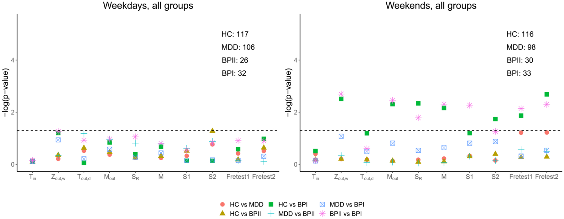
Comparison of activity distributions among the healthy controls (HC), MDD, BPI, and BPII individuals for activities on weekdays and on weekends. For each individual, seven weekdays and three weekends of data are used. The $-\text{log}(p-\mathit{\text{values}})$ are plotted for each of the proposed test statistics, the generalized edge-count tests $(S1,S2)$ and Fréchet tests (Fretest1, Fretest2). The corresponding sample size for each group is presented on the upper right corner.

5.2. Comparison of activity distributions among different age groups.

It is well known that age is associated with the amount of physical activity. For example, Schrack et al. (2014) found “a 1.3% decrease per year” in cumulative physical activity counts from mid-to-late life among an elderly population. Similar results have been reported in several other large cohort studies and age groups, including NHANES and UK Biobank (Doherty et al. (2017), Varma et al. (2017), Viciana, Mayorga-Vega and Martínez-Baena (2016)). However, few studies have examined how inter- and intra-individual variability in physical activity differs by age. We ask whether the proposed test statistics are able to detect differences in the daily activity densities over different age categories and inform us where the difference lies. To ensure a proper power with an adequate sample size, we take the two diagnostic groups with the largest sample sizes, the HC and major depressive disorder (MDD), and stratify them into three age groups: young (age ≤ 30), middle age (30 < age ≤ 60), and older age (age > 60) groups. We also separately test activity densities from weekdays and weekends.

The $p$-values of the proposed test statistics, the generalized edge-count test $(S1,S2)$, and Fréchet test (Fretest1, Fretest2) are shown in Figure 5 with detailed $p$-values given in Table 6 of the Supplementary Material. Overall, among the healthy individuals, the proposed tests find large differences in the distributions of activity intensities among the three age groups for both weekdays and weekends. Such differences are especially prominent when comparing the young age group or middle age group with the older group during the weekdays. In contrast, Fréchet test fails to detect such differences in most of the comparisons and is only able to capture marginally significant results when comparing the young and older individuals among MDD patients. The tests $S1$ and $S2$ also show fewer significant results than our proposed tests.

Fig. 5.

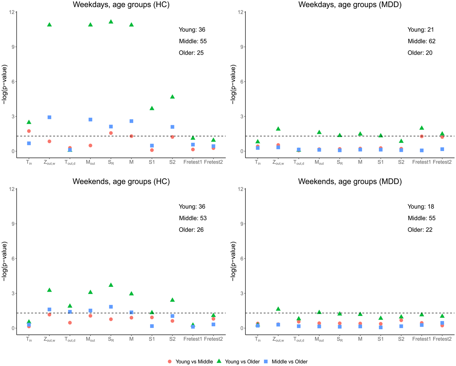
Comparison of activity distributions in different age groups for young (≤ 30), middle (30 < age ≤ 60), and older age (> 60) groups. The $-\text{log}(p-\mathit{\text{values}})$ of the proposed test statistics, the generalized edge-count tests $(S1,S2)$, and Fréchet tests (Fretest1, Fretest2) are presented for different comparisons. The corresponding sample size for each group is presented on the upper-right corner.

To further demonstrate the possible gain of power, we note that, among the patients with MDD, only the proposed $Z_{\text{out,}w}$ test shows statistically significant difference between young and older groups for both weekend and weekday activities. Fréchet test shows some difference in activity distributions between young and older groups but only for the weekdays. To confirm the detected differences in the original data, we visualize the density data in Figure 6 by projecting them onto lower-dimensional plots, using multidimensional scaling (MDS), based on the Wasserstein distances. The figure clearly shows difference in activity densities between young and older groups for both weekdays and weekends among MDD patients.

Fig. 6.

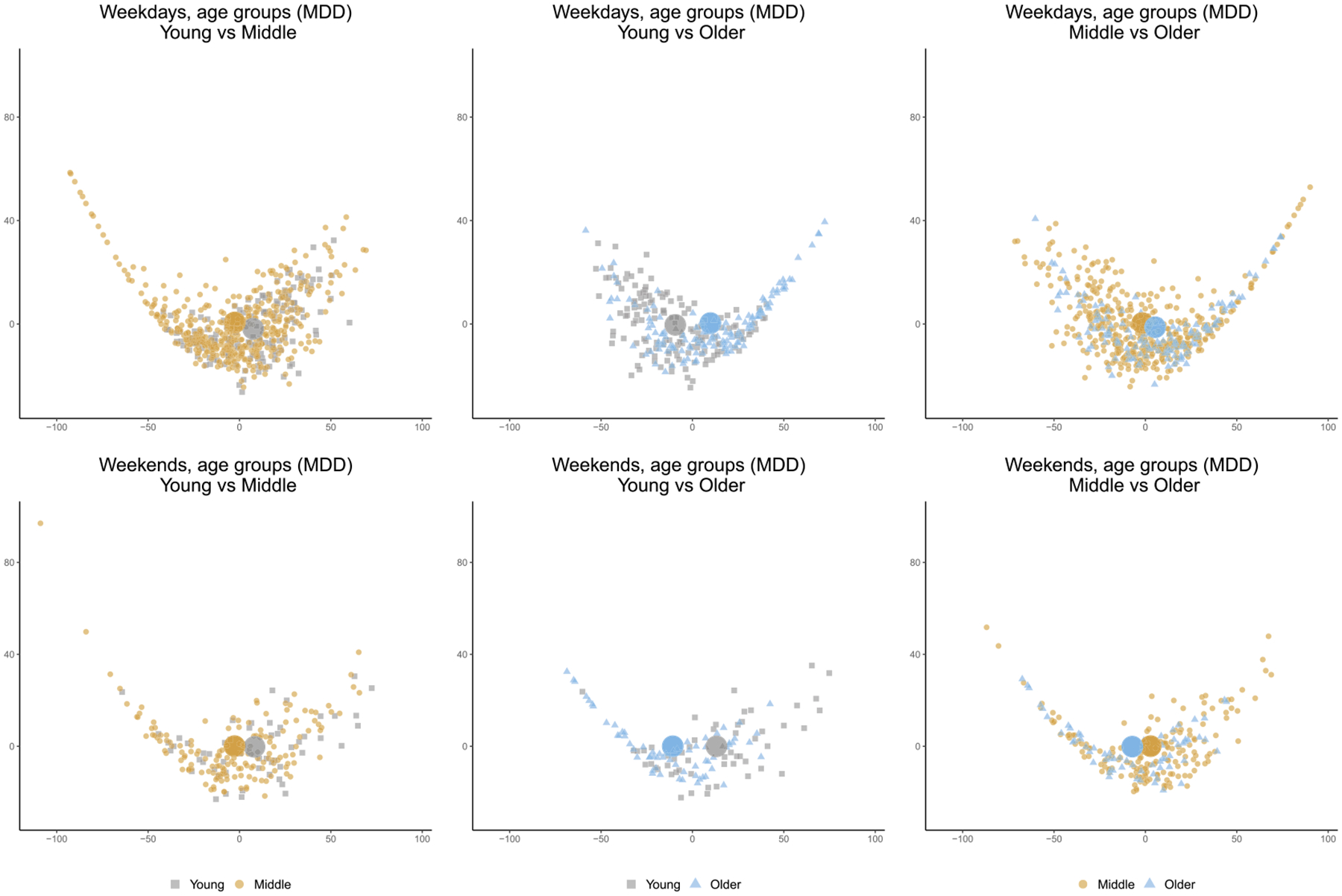
Multidimensional scaling (MDS) plots based on the Wasserstain distances to visualize the distribution of activity densities among MDD patients, across three pairwise comparisons by age groups (left, middle, right) and on weekdays (top) and weekends (bottom).

Finally, it is also interesting that $T_{\text{in}}$ detects significant difference in day-to-day variability between the healthy young group and older group on weekdays. In fact, we obtained a negative value for $Z_{\text{in}}$ which implies that the younger subjects have larger day-to-day variability than the older subjects. Lastly, $T_{\text{out},\text{d}}$ does not yield any significant results in most cases, indicating that there is large subject heterogeneity within each age group, yet their scales are comparable.

5.3. Comparison of activity distributions among different BMI groups.

A third factor that could potentially affect differential physical activity patterns is the body mass index (BMI). We apply our proposed tests to examine difference in daily activity density among individuals who are lean with BMI ≤ 25 and obese with BMI > 25 among healthy individuals and those with mood disorders (OTHER). To control for the age effect, we only consider those individuals with age of 30 years or older.

The results are provided in Figure 7. Among the healthy individuals, little difference is observed in their activity distribution patterns between lean and obese individuals during the weekdays and weekends. When assessing among patients in the OTHER group, we observe some differences in the mean of the activity distributions both during weekdays and weekends. We do not see group differences in the within-individual or between-individual variability. The generalized edge-count test and Fréchet test achieve nonsignificant large $p$-values and fail to reject the null hypothesis for all the comparisons. This further demonstrates that our proposed test statistics can detect difference in activities that could be missed by other methods.

Fig. 7.

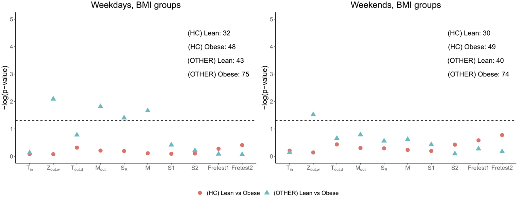
Comparison of activity distributions by BMI (lean and obese groups). The $-\text{log}(p-\mathit{\text{values}})$ of the proposed test statistics, the generalized edge-count tests $(S1,S2)$, and Fréchet tests (Fretest1, Fretest2) are presented for different comparisons. The corresponding sample size for each group is presented on the upper-right corner.

6. Discussion.

In this paper, we have extended the graph-based two-sample tests for density data and proposed several test statistics to account for repeated measures data by considering both the within-individual similarity graph $G_{\text{in}}$ and between-individual similarity graph $G_{\text{out}}$ The graph allows for more than one edge between any two individuals which extends the existing graph-based testing methods where only one edge between any two individuals is allowed. We have proposed a list of six test statistics that capture different alternatives that are associated with distributions of density functions, including differences in mean, inter- and intra-individual variances. These statistics are constructed based on the similarity graph $G$ which is the union of $G_{\text{in}}$ and $G_{\text{out}}$. Furthermore, we have developed the asymptotic null distributions that can be used to obtain $p$-values under the permutation null. The test statistics are easy to calculate, and the testing procedures are computationally efficient. Our simulation studies have shown that the proposed test statistics control the desired type 1 errors and are more powerful than existing distance-based tests that ignore the repeated observations.

In our analysis of the physical activity measures with repeated observations, we have observed a substantial differences in the day-to-day variability within subject across disease groups and age categories. Such findings have rarely been reported previously. Our proposed tests are able to take into account such within-individual dependency and variability. Compared to the two versions of Fréchet tests, we observed increased power in detecting the differences in activity densities. In addition, by comparing results utilizing various proposed test statistics, we are able to further understand the complex data structures and decompose the source of differences between various groups.

Our proposed permutation procedure treats the entire vector of repeated observations of objects from an individual as the independent unit which requires that we have the same number of observations for each individual. Otherwise, the within-individual Wasserstein covariance is not well defined. This approach eliminates any assumptions on the errors of the repeated measures. For example, we do not require that the repeated measures have the same marginal distribution and allow them to be different from day to day. In our analysis of the NIMH physical activity data, we noticed that the results are robust to different subsets of the observations used in our analysis and reported an average through Fisher’s transformation. However, there might be the case when an unequal number of repeated observations might be informative, in which case one should interpret the results with care. An interesting future research topic is to extend the proposed tests to allow for different numbers of repeated observations by making additional assumptions on these repeated measures.

REFERENCES

- Banda JA, Haydel KF, Davila T, Desai M, Bryson S, Haskell WL, Matheson D and Robinson TN (2016). Effects of varying epoch lengths, wear time algorithms, and activity cut-points on estimates of child sedentary behavior and physical activity from accelerometer data. PLOS ONE 11 e0150534. [DOI] [PMC free article] [PubMed] [Google Scholar]
- Burton C, McKinstry B, Tătar AS, Serrano-Blanco A, Pagliari C and Wolters M (2013). Activity monitoring in patients with depression: A systematic review. J. Affective Disorders 145 21–28. [DOI] [PubMed] [Google Scholar]
- Chapman JJ, Roberts JA, Nguyen VT and Breakspear M (2017). Quantification of free-living activity patterns using accelerometry in adults with mental illness. Sci. Rep 743174. [DOI] [PMC free article] [PubMed] [Google Scholar]
- Chen H, Chen X and Su Y (2018). A weighted edge-count two-sample test for multivariate and object data. J. Amer. Statist. Assoc 113 1146–1155. 10.1080/01621459.2017.1307757 [DOI] [Google Scholar]
- Chen H and Friedman JH (2017). A new graph-based two-sample test for multivariate and object data. J. Amer. Statist. Assoc 112 397–409. 10.1080/01621459.2016.1147356 [DOI] [Google Scholar]
- Crescenzo FD, Economou A, Sharpley AL, Gormez A and Quested DJ (2017). Actigraphic features of bipolar disorder: A systematic review and meta-analysis. Sleep Med. Rev 33 58–69. 10.1016/j.smrv.2016.05.003 [DOI] [PubMed] [Google Scholar]
- Dawson JD and Lagakos SW (1993). Size and power of two-sample tests of repeated measures data. Biometrics 49 1022–1032. 10.2307/2532244 [DOI] [PubMed] [Google Scholar]
- Doherty A, Jackson D, Hammerla N, Plötz T, Olivier P, Granat MH, White T, van Hees VT, Trenell MI et al. (2017). Large scale population assessment of physical activity using wrist worn accelerometers: The UK biobank study. PLoS ONE 12 e0169649. 10.1371/journal.pone.0169649 [DOI] [PMC free article] [PubMed] [Google Scholar]
- Dubey P and Müller H-G (2019). Fréchet analysis of variance for random objects. Biometrika 106 803–821. 10.1093/biomet/asz052 [DOI] [Google Scholar]
- Faurholt-Jepsen M, Brage S, Vinberg M, Christensen EM, Knorr U, Jensen HM and Kessing LV (2012). Differences in psychomotor activity in patients suffering from unipolar and bipolar affective disorder in the remitted or mild/moderate depressive state. J. Affective Disorders 141 457–463. 10.1016/j.jad.2012.02.020 [DOI] [PubMed] [Google Scholar]
- Friedman JH and Rafsky LC (1979). Multivariate generalizations of the Wald-Wolfowitz and Smirnov two-sample tests. Ann. Statist 7 697–717. [Google Scholar]
- Gretton A, Borgwardt KM, Rasch MJ, Schölkopf B and Smola A (2012). A kernel two-sample test. J. Mach. Learn. Res 13 723–773. [Google Scholar]
- Henze N (1988). A multivariate two-sample test based on the number of nearest neighbor type coincidences. Ann. Statist 16 772–783. 10.1214/aos/1176350835 [DOI] [Google Scholar]
- Indic P, Salvatore P, Maggini C, Ghidini S, Ferraro G, Baldessarini RJ and Murray G (2011). Scaling behavior of human locomotor activity amplitude: Association with bipolar disorder. PLoS ONE 6 e20650. 10.1371/journal.pone.0020650 [DOI] [PMC free article] [PubMed] [Google Scholar]
- Keadle SK, Shiroma EJ, Freedson PS and Lee IM (2014). Impact of accelerometer data processing decisions on the sample size, wear time and physical activity level of a large cohort study. BMC Public Health 14 1210. 10.1186/1471-2458-14-1210 [DOI] [PMC free article] [PubMed] [Google Scholar]
- Krane-Gartiser K, Henriksen TEG, Morken G, Vaaler A and Fasmer OB (2014). Actigraphic assessment of motor activity in acutely admitted inpatients with bipolar disorder. PLOS ONE 9 e89574. [DOI] [PMC free article] [PubMed] [Google Scholar]
- Leeger-Aschmann CS, Schmutz EA, Zysset AE, Kakebeeke TH, Messerli-Bürgy N, Stülb K, Arhab A, Meyer AH, Munsch S et al. (2019). Accelerometer-derived physical activity estimation in preschoolers-comparison of cut-point sets incorporating the vector magnitude vs the vertical axis. BMC Public Health 19513. [DOI] [PMC free article] [PubMed] [Google Scholar]
- Merikangas KR, Cui L, Heaton L, Nakamura E, Roca C, Ding J, Qin H, Guo W, Shugart YY et al. (2014). Independence of familial transmission of mania and depression: Results of the NIMH family study of affective spectrum disorders. Mol. Psychiatry 19 214–9. 10.1038/mp.2013.116 [DOI] [PubMed] [Google Scholar]
- Merikangas KR, Swendsen J, Hickie IB, Cui L, Shou H, Merikangas AK, Zhang J, Lamers F, Crainiceanu C et al. (2019). Real-time mobile monitoring of the dynamic associations among motor activity, energy, mood, and sleep in adults with bipolar disorder. JAMA Psychiatr. 76 190–198. [DOI] [PMC free article] [PubMed] [Google Scholar]
- Murray G, Gottlieb J, Hidalgo MP, Etain B, Ritter P, Skene DJ, Garbazza C, Bullock B, Merikangas K et al. (2020). Measuring circadian function in bipolar disorders: Empirical and conceptual review of physiological, actigraphic, and self-report approaches. Bipolar Disorders. 10.1111/bdi.12963 [DOI] [PubMed] [Google Scholar]
- Pagani L, Clair PAS, Teshiba TM, Service SK, Fears SC, Araya C, Araya X, Bejarano J, Ramirez M et al. (2016). Genetic contributions to circadian activity rhythm and sleep pattern phenotypes in pedigrees segregating for severe bipolar disorder. Proc. Natl. Acad. Sci. USA 113 E754–E761. 10.1073/pnas.1513525113 [DOI] [PMC free article] [PubMed] [Google Scholar]
- Petersen A and Müller H-G (2019). Wasserstein covariance for multiple random densities. Biometrika 106 339–351. 10.1093/biomet/asz005 [DOI] [Google Scholar]
- Robillard R, Hermens DF, Naismith SL, White D, Rogers NL, Ip TKC, Mullin SJ, Alvares GA, Guastella AJ et al. (2015). Ambulatory sleep-wake patterns and variability in young people with emerging mental disorders. J. Psychiatry Neurosci 40 28–37. 10.1503/jpn.130247 [DOI] [PMC free article] [PubMed] [Google Scholar]
- Rosenbaum PR (2005). An exact distribution-free test comparing two multivariate distributions based on adjacency. J. R. Stat. Soc. Ser. B. Stat. Methodol 67 515–530. 10.1111/j.1467-9868.2005.00513.x [DOI] [Google Scholar]
- Schilling MF (1986). Multivariate two-sample tests based on nearest neighbors. J. Amer. Statist. Assoc 81 799–806. [Google Scholar]
- Schott JR (2007). A test for the equality of covariance matrices when the dimension is large relative to the sample sizes. Comput. Statist. Data Anal 51 6535–6542. 10.1016/j.csda.2007.03.004 [DOI] [Google Scholar]
- Schrack JA, Zipunnikov V, Goldsmith J, Bai J, Simonsick EM, Crainiceanu C and Ferrucci L (2014). Assessing the “physical cliff”: Detailed quantification of age-related differences in daily patterns of physical activity. J. Gerontol., Ser. A, Biol. Sci. Med. Sci 69 973–9. 10.1093/gerona/glt199 [DOI] [PMC free article] [PubMed] [Google Scholar]
- Schrack JA, Cooper R, Koster A, Shiroma EJ, Murabito JM, Rejeski WJ, Ferrucci L and Harris TB (2016). Assessing daily physical activity in older adults: Unraveling the complexity of monitors, measures, and methods. J. Gerontol., Ser. A, Biol. Sci. Med. Sci 71 1039–1048. 10.1093/gerona/glw026 [DOI] [PMC free article] [PubMed] [Google Scholar]
- Scott J, Murray G, Henry C, Morken G, Scott E, Angst J, Merikangas KR and Hickie IB (2017). Activation in bipolar disorders: A systematic review. JAMA Psychiatr. 74 189–196. 10.1001/jamapsychiatry.2016.3459 [DOI] [PubMed] [Google Scholar]
- Shou H, Cui L, Hickie I, Lameira D, Lamers F, Zhang J, Crainiceanu C, Zipunnikov V and Merikangas KR (2017). Dysregulation of objectively assessed 24-hour motor activity patterns as a potential marker for bipolar I disorder: Results of a community-based family study. Translational Psychiatry 7 e1211. 10.1038/tp.2017.136 [DOI] [PMC free article] [PubMed] [Google Scholar]
- Varma VR, Dey D, Leroux A, Di J, Urbanek J, Xiao L and Zipunnikov V (2017). Re-evaluating the effect of age on physical activity over the lifespan. Prev. Med 101 102–108. 10.1016/j.ypmed.2017.05.030 [DOI] [PMC free article] [PubMed] [Google Scholar]
- Varma VR, Dey D, Leroux A, Di J, Urbanek J, Xiao L and Zipunnikov V (2018). Total volume of physical activity: TAC, TLAC or TAC(λ). Prev. Med 106 233–235. 10.1016/j.ypmed.2017.10.028 [DOI] [PMC free article] [PubMed] [Google Scholar]
- Viciana J, Mayorga-Vega D and Martínez-Baena A (2016). Moderate-to-vigorous physical activity levels in physical education, school recess, and after-school time: Influence of gender, age, and weight status. J. Phys. Act. Health 13 1117–1123. 10.1123/jpah.2015-0537 [DOI] [PubMed] [Google Scholar]
- Wrobel J, Zipunnikov V, Schrack J and Goldsmith J (2019). Registration for exponential family functional data. Biometrics 75 48–57. 10.1111/biom.12963 [DOI] [PMC free article] [PubMed] [Google Scholar]
- Yang H, Baladandayuthapani V, Rao AUK and Morris JS (2020). Quantile function on scalar regression analysis for distributional data. J. Amer. Statist. Assoc 115 90–106. 10.1080/01621459.2019.1609969 [DOI] [PMC free article] [PubMed] [Google Scholar]
- Zhang J and Chen H (2022). Graph-based two-sample tests for data with repeated observations. Statist. Sinica 32 391–415. 10.5705/ss.202019.0116 [DOI] [Google Scholar]
- Zhang J, Merikangas KR, Li H and Shou H (2022). Supplement to “Two-sample tests for multivariate repeated measurements of histogram objects with applications to wearable device data.” 10.1214/21-AOAS1596SUPP [DOI] [PMC free article] [PubMed] [Google Scholar]
Associated Data
This section collects any data citations, data availability statements, or supplementary materials included in this article.