Figure 3.
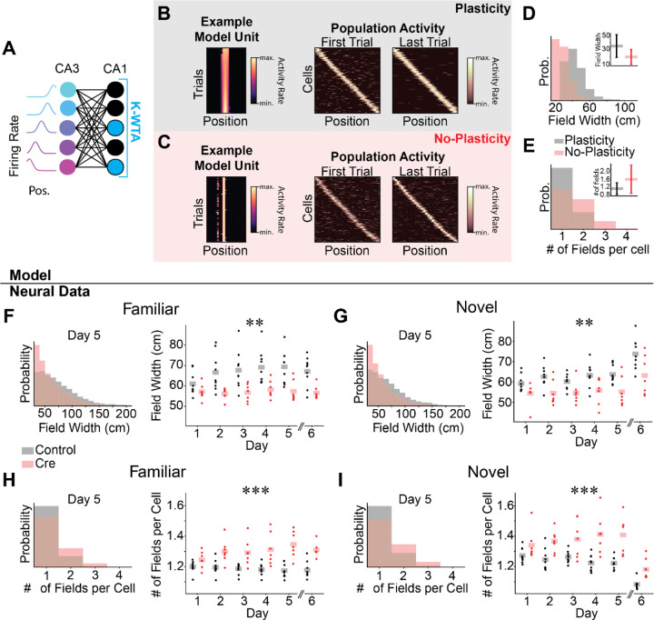
Spatial coding in Cre animals may be passively inherited from upstream activity. A-E) Computational model of the CA3-CA1 circuit.
A) Schematic for K-Winners-Take-All (KWTA) model of place field inheritance. A set of place selective cells (“CA3”) projects randomly to a set of output neurons (“CA1”). The set of active neurons at the output layer at each position is determined by a KWTA threshold (the K most excited neurons are active [blue], all other neurons are silent [black]). In the “Plasticity” model, synaptic weights are updated according to a noisy Hebbian rule. In the “No-Plasticity” model, synaptic weights randomly fluctuate.
B-C) Both the Plasticity and No-Plasticity models produce stable place cells at the CA1 layer.
B) Plasticity model spatial coding. Left - Position-binned activity of an example place selective unit from the model. Each row is a single training iteration of the model, akin to a trial in the real experiment. Columns indicate virtual position. Middle & Right - The activity of all place selective units is plotted for the first (Middle) and last trial (Right). Model cells are sorted by their location of peak activity on the last trial. Each row indicates the z-scored activity rate of a unit as a function of position.
C) Same as (B) for the No-Plasticity model. Note similar spatial coding and stability in the two models.
D) Place fields are wider in the Plasticity model. Histogram of place field widths (black - Plasticity, red - No-Plasticity). Inset - mean ± std field width from each model.
E) The Plasticity model has fewer place fields per cell than the No-Plasticity model. Histogram of the number of place fields per cell (black - Plasticity, red - No-Plasticity). Inset - mean ± std number of fields per cell from each model.
F-I) Differences between Control and Cre animal place field properties mirror differences between Plasticity and No-Plasticity models.
F-G) Cre animals have narrower place fields.
F) Familiar trials. Left - Histogram of place field widths for combined data from day 5 (black - Control, red - Cre). Right - Within animal average field width on each day. Dots indicate the across cell average for each mouse. Shaded bars indicate across animal means. [N=9 control mice, 7 Cre mice, 5 days (day 6 excluded). Mixed effects ANOVA: virus main effect F(1,14)=10.6 p=.006, day main effect F(4, 56)=4.57 p=0.003, interaction F(4,56)=2.81 p=0.034; day 6 unpaired t-test control vs Cre: t=−3.90 p=.002]
G) Same as (F) for novel trials. [N=9 control mice, 7 Cre mice, 5 days (day 6 excluded). Mixed effects ANOVA: virus main effect F(1,14)=10.2 p=.007, day main effect F(4,56)=2.11 p=.091, interaction F(4,56)=.758 p=.557; day 6 unpaired t-test control vs Cre: t=−2.38 p=.036]
H-I) Cre animals have more place fields per cell.
H) Familiar trials. Left - Histogram of number of place fields per cell for day 5 data combined across all mice (Control - black, Cre-red). Right - Within animal average number of place fields per cell on each day. Dots indicate the across cell average for each mouse. Shaded bars indicate across animal means. [N=9 control mice, 7 Cre mice, 5 days (day 6 excluded). Mixed effects ANOVA: virus main effect F(1,14)=25.5 p=1.76×10⁻⁴, day main effect F(4,56)=.804 p=.528, interaction F(4,56)=3.29 p=.017; day 6 unpaired t-test control vs Cre: t=5.30 p=1.19×10⁻⁴].
I) Same as (H) for novel trials [N=9 control mice, 7 Cre mice, 5 days (day 6 excluded). Mixed effects ANOVA: virus main effect F(1,14)=17.5 p=9.12×10⁻⁴, day main effect F(4,56)=.158 p=.959, interaction F(4,56)=2.96 p=0.027; day 6 unpaired t-test control vs Cre: t=3.52 p=.008]
See also Figure S5.

