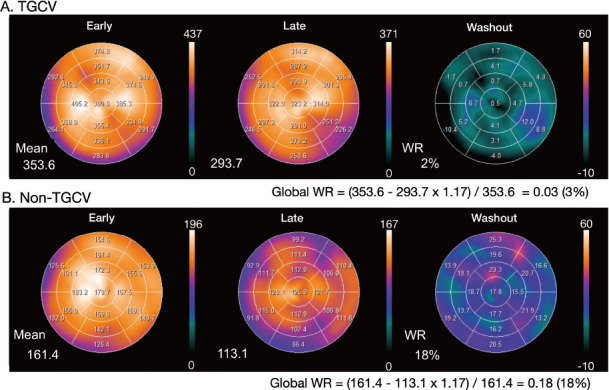
Figure 3 Examples of WRs in SPECT polar maps.

A: Clinical diagnosis of TGCV with WR 3%.

B: Coronary artery disease with WR 18%. Late image is shown with color scale in which maximum count is multiplied by a time-decay correction factor of 3 h (1.17). Global WR can be calculated by defining WR (Eq. 1) after decay correction. Compared with average of pixel-based WR (left lower corner of WR polar map, 2%), global WR (3%) was in agreement when regional WR values were homogeneous. However, averaged pixel-based WR might be influenced by misaligned early and late slices or defective regions.

WRs, washout rates.