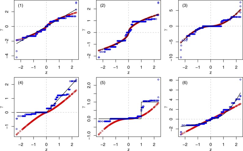
Figure 1.

Final prior effects $\mathit{\gamma }$ (y-axis) against initial prior effects z (x-axis), under exponential calibration (red points on continuous curve) and isotonic calibration (blue points on discontinuous curve). The thin black line corresponds to perfect calibration ($\mathit{\gamma }=\mathit{\beta }$). We simulated the feature matrix X from a standard Gaussian distribution (n = 200, p = 500) and the initial prior effects z from a trimmed standard Gaussian distribution (trimmed below the 1% and above the 99% quantile). We set the true coefficients to (1)$\mathit{\beta }=\mathit{z}$, (2)$\mathit{\beta }=\text{sign}(\mathit{z})\sqrt{\left|\mathit{z}\right|}$, (3)$\mathit{\beta }=\text{sign}(\mathit{z}){\mathit{z}}^2$, (4)$\mathit{\beta }=\mathbb{I}[\mathit{z}>0]\mathit{z}$, (5)$\mathit{\beta }=\mathbb{I}[\mathit{z}>1]$, or (6)$\mathit{\beta }=-\mathbb{I}[\mathit{z}\le 0]\sqrt{\left|\mathit{z}\right|}+\mathbb{I}[\mathit{z}>0]{\mathit{z}}^2$. And we simulated the response vector y from Gaussian distributions with the means $\mathit{\eta }$ and the variance $\text{Var}(\mathit{\eta })$, where $\mathit{\eta }=\mathit{X\beta }$. While exponential calibration performs slightly better in the first three scenarios (top), isotonic calibration performs much better in the last three scenarios (bottom).