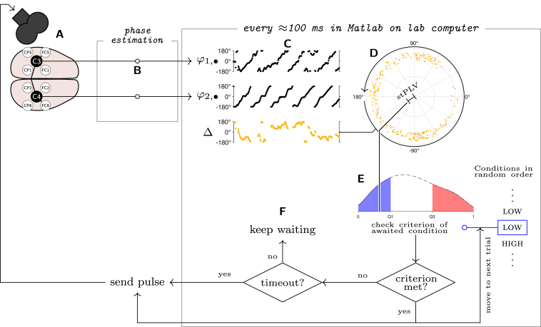
Fig. 1.

Overview of the closed-loop EEG-TMS setup: the signal from the C3- and C4-Hjorth montages was recorded (A), and processed in real time by the bossdevice (B), which yielded the estimated instantaneous phases from the last 500 ms (250 samples, ${\phi }_{1,1},\dots {\phi }_{1,N},{\phi }_{2,1},\dots ,{\phi }_{2,N}$ in Eq. (1)). The phase estimates were retrieved by the controlling PC, and the instantaneous phase differences ($\Delta$) were computed (C). From these, the single-trial PLV was obtained as the magnitude of the complex-valued average of the phase-difference phasors (all of unit length, here jittered for readability; D). The current stPLV was then compared against the criterion of the current condition (E). In the visualized case, the current condition is low, so the current stPLV is compared to the lower quartile of the empirical stPLV-distribution. If the stPLV is below the low-condition threshold, a pulse was sent, followed by a 2 s pause (minISI$=2$ s), and the system proceeded to wait for the next condition (here: high). If the criterion was not met, the system checked whether the time since the last stimulus exceeded 8 s – if it did, a timeout pulse was sent, followed by the 2-s minISI pause — but the condition was not updated. If timeout had not been reached, the system simply kept waiting (F). When waiting, the 500 ms windows of phases were retrieved (roughly) every 100 ms. Every computed stPLV was also added to the empirical stPLV-distribution (E) after comparing it to the current criterion, replacing the oldest stPLV — then, the criteria were recomputed.