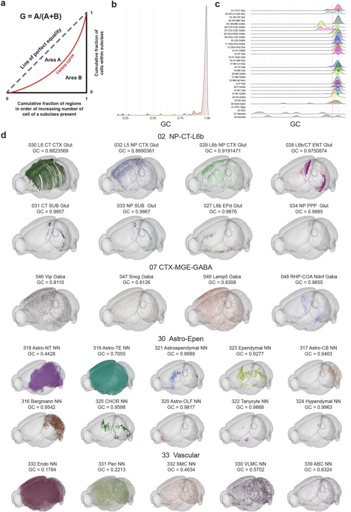
Extended Data Fig. 14. Distribution of Gini coefficient for subclasses.
(a) Illustration explaining the concept of the Gini coefficient (GC). For each subclass, brain regions are ordered by number of cells present in x-axis. The y-axis is the cumulative fraction of cells for each subclass. The Gini coefficient is calculated by dividing the area (Area A) between the line of perfect equality and the observed distribution curve (the Lorenz curve) by the total area under the line of perfect equality (Areas A + B). The result is a value between 0 and 1 with 0 representing perfect equality and 1 maximum inequality. (b) Distribution of GCs for all subclasses. Color scheme is the same as used for Fig. 6a. (c) Ridge plot showing the distribution of GCs for subclasses grouped by class. (d) 3D example plots of subclasses for 4 classes (02 NP-CT-L6b, 07 CTX-MGE-GABA, 30 Astro-Epen, and 33 Vascular), illustrating the wide range of GCs present. Within each class, plots are ordered by GC from lowest to highest.

