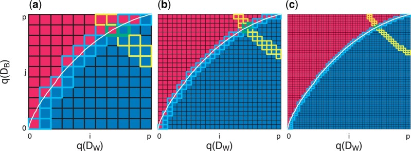
Fig. 4.
Graphical representation of two HPE algorithms to estimate  . We simulate observations from two Gaussian distributions, namely
  and
and  and calculate the quantiles
  and
and  for each of the sets with (a)
  , (b)
, (b)  , and (c)
  . The white curve represents the percent of elements in
  that are strictly less than each element in
  . The goal is to estimate the true
  (area under the white curve) using one of two HPE algorithms. The brute force approach (HPE algorithm 1) uses Riemann integration to approximate the white curve by summing the area of the blue squares below the curve. The grid search approach (HPE algorithm 2) starts at the minimum of
  and
and  and moves along the red–blue border to approximate the white curve (path followed represents the squares with the light blue borders). The HPE contour
  (or estimate of
  )
)  is given by yellow-bordered squares. In other words, every pair
  such that
  , the interval guaranteed to contain
  . The intersection of this yellow contour (
 ) and blue contour (grids visited by HPE algorithm 2) are the green-bordered squares, which represents the numerical estimate for
  and
and  .
.

