Figure 3.

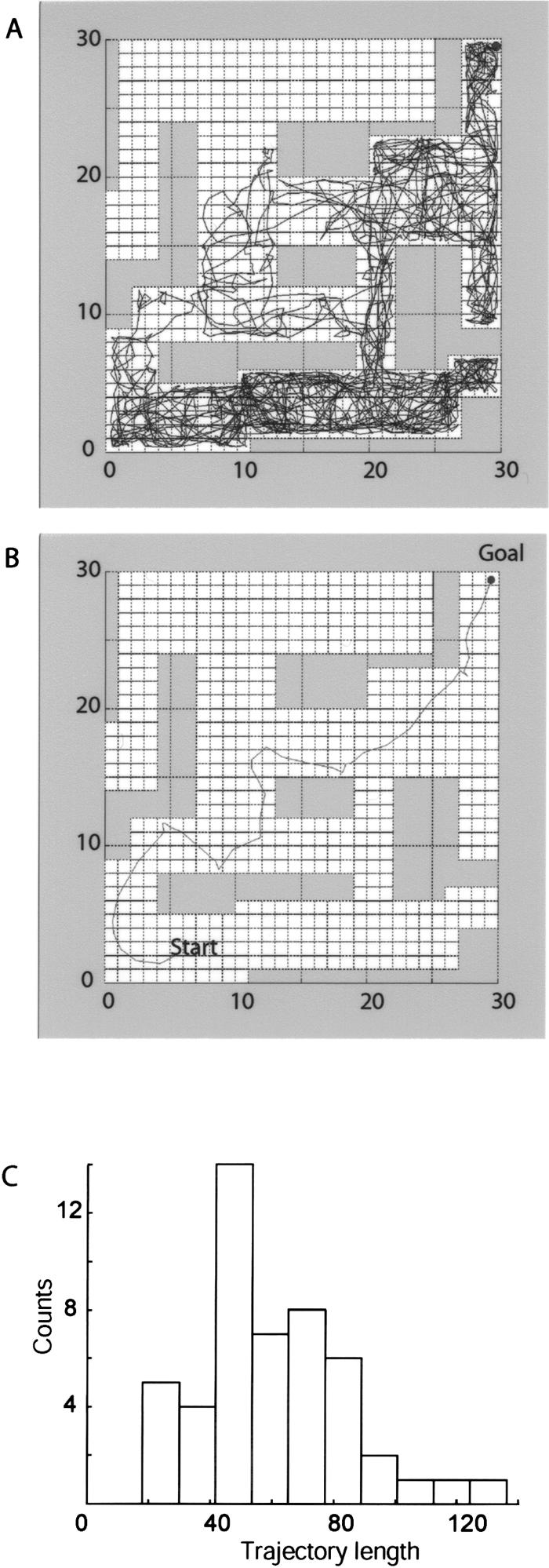
Simulation results for two-dimensional navigation. (A) A sample random trajectory during exploration of the maze. The CA1 unit subsequently selected as a goal represents the top, right corner square (black dot). Each square of the lattice corresponds to one CA3 unit of the model network that is a discrete graph; however, the simulated motion is continuous. The exploratory motion is controlled by equation 2 with randomly fluctuating acceleration a. The trajectory does not cover the maze uniformly; in fact, a large part of the maze remains unexplored (top, left area). The running starts at the bottom of the maze and is continued until the future goal location is reached. (B) A sample trajectory toward the goal following the learning session shown in A. In this case, the acceleration a in equation 2 is controlled by the model (Fig. 2) according to the algorithm described in the text. The trajectory in B is reasonably close by its length to a shortest path and is ∼60 times shorter than a typical random walk, e.g., the trajectory in A. (C) Histogram of goalsearch trajectory lengths for the learning scenario represented in A. The units of length correspond to those of A and B.