Figure 1.

Examples of EBSD maps and their interpretation

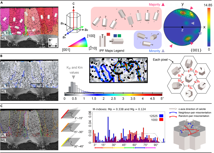
(A) Inverse Pole Figure (IPF) map showing calcite grains, from the Palisade Layer (PL), colored with the IPF map component. Grains with their c-axis that tend to be perpendicular to the eggshell surface (parallel to y-direction) are colored in reddish tones (majority); whereas the grains that tend to be parallel to the eggshell surface (x-, z-directions) are colored in greenish and bluish tones (minority). The majority reddish grains contribute to the hotspots of {001} pole figures at the polar regions. The minority bluish and greenish grains contribute to the weak signals at the equatorial parts of the pole figure. The value above the color bar (14.85) represents the multiple of uniform distribution density (MUD) value (high MUD value indicates strong crystallographic alignment and MUD value of 1 represents random distribution). Transverse direction Kearns texture factors (f_T) values were extracted from {001} pole figures. The pfJ-index values were extracted from {001}, {2$\overline{1}$0} and {100} pole figures.

(B) Kernel Average Misorientation (KAM) map identifying regions with KAM values between 0° (grayish tones) and 5° (dark reddish tones). These values represent the misorientation calculated by mean orientation between a point and its designated number of neighboring pixels, mapped according to the colored scale (KAM value = mean{θ_i, 1 ≤ i ≤ 6}). The set of all these KAM values for a studied sample is shown in a frequency distribution histogram (central schematic). From the histogram, we obtain the average and median KAM values (Kμ and Km) per eggshell sample.

(C) On a grain boundary (GB) map, misorientation angles between grains are represented by colors: 3° < θ ≤ 15° in red, 15° < θ ≤ 30° in orange, 30° < θ ≤ 45° in yellow, 45° < θ ≤ 60° in green, 60° < θ ≤ 75° in blue, and 75° < θ ≤ 90° in purple. The frequency distribution of (neighbour-pair and random-pair) misorientation is represented as a histogram. The continuous curve on the histogram shows the theoretical random distribution. The numbers next to blue and red boxes show the number of neighbour-pair (correlated) and random-pair (uncorrelated) misorientations. M-indexes (Mp and Mg) are defined on the base of the distribution of uncorrelated misorientation angles and theoretical random distribution. Legend, PL: Palisade Layer, ML: Mammillary Layer. For additional information, see STAR Methods.