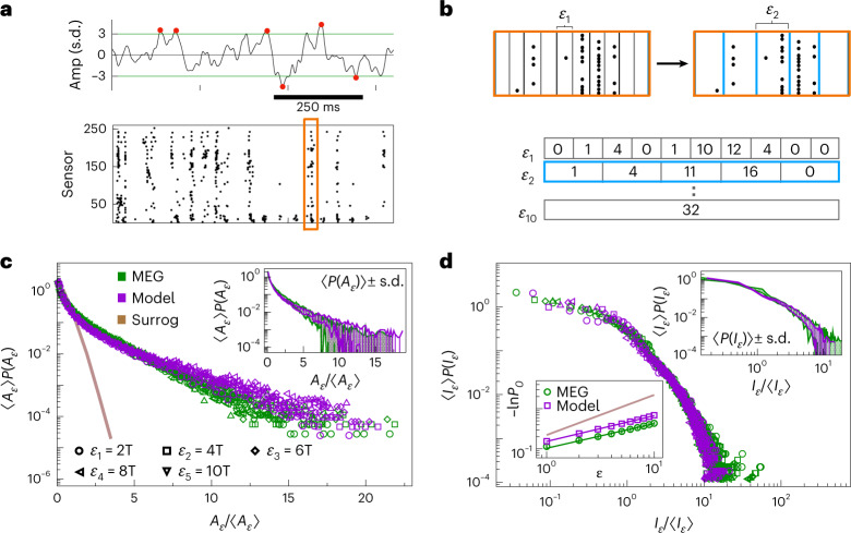
Fig. 3. Connecting non-exponential extreme event statistics in MEG resting-state activity and in a marginally subcritical adaptive Ising model.
a, Top: extreme events identified on a single sensor (red dots) using e = ± 3 s.d. (horizontal lines). Bottom: the resulting raster of extreme events shown across 273 MEG sensors of a single subject. b, Top: Aϵ is defined as the total number of extreme events across all sensors in a time bin ϵn = nT, a multiple of the sampling interval T. Bottom: representative sequences of network excitation extracted from the raster in the top panel for increasing ϵn. c, Rescaled distributions P(Aϵ) for a range of ϵn (different plot symbols) collapse onto a single non-exponential master curve for both the data (green symbols represent the average over subjects) and model simulated at baseline parameters, with K = 100 subsystems of nsub = 1,000 neurons each (violet symbols) (N = 105). The corresponding distribution in phase-scrambled MEG signals shows an exponential behavior, with absence of high excitation events (the brown line represents surrogate data). Inset: rescaled P(Aϵ) (green symbols represent the average over n = 14 MEG subjects, whereas violet symbols represent the average over the model simulations) and respective s.d. (colored areas) shown for ϵ = 2T. d, Rescaled distributions of quiescence durations, P(Iϵ) collapse onto a single master curve for different values of ϵ. The plotting conventions and model simulation details are the same as in c. Top inset: rescaled P(Iϵ) (green symbols represent the average of n = 14 MEG subjects, whereas violet symbols are the average over model simulations) and respective s.d. (colored area) shown for ϵ = 2T. Bottom inset: the probability P0 of finding a quiescent time bin approximately scales as with ϵ; βI = 0.582 ± 0.013 and βI = 0.610 ± 0.012 for the data and model, respectively; βI = 0.996 ± 0.001 for surrogate data. The exponent βI was estimated via an ordinary linear least-square fit y = ax + b, where and .

