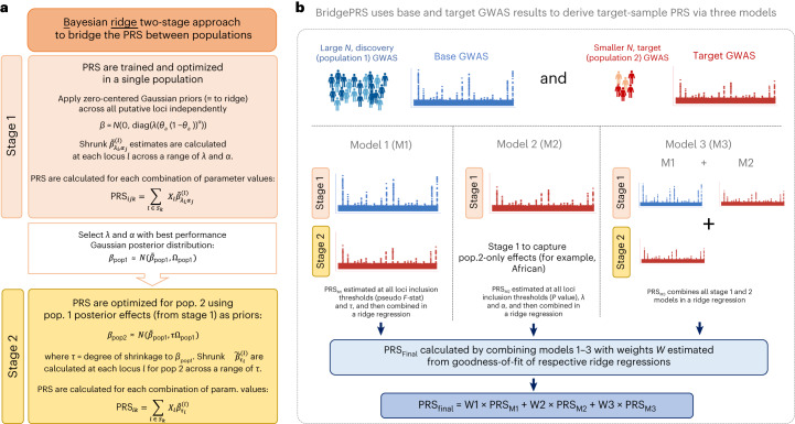
Fig. 1. Flow diagram describing the modeling of BridgePRS.

a, Two-stage approach to combine GWASs from two populations. b, BridgePRS combining three different PRS models to determine the final PRS. β, SNP effect sizes; λ, shrinkage coefficients; θ_a, allele frequency of SNP a; α, parameter for dependency between effect size and allele frequency; τ, degree of shrinkage of population 2 effects, β_pop2, to those of population 1, β_pop1; X_l, genotypes at locus l, where a locus is defined as a region in which SNPs are correlated (r² > 0.01) with each other; ${\tilde{\mathbf{\beta }}}^{\left(l\right)}$, posterior mean SNP effects at locus l, where subscripts denote prior parameters used; Ω_pop1, posterior precision matrix for population 1 using the best-fitting prior parameters α and λ (the Gaussian distribution is parameterized by its precision matrix (inverse covariance matrix), throughout). S_k is the set of loci whose rank exceeds a threshold of k: in stage 1 loci are ranked by the P value of their top SNP, whereas in stage 2 loci are ranked by the pseudo F statistic, which measures the joint association of all SNPs at the locus in the target population; i and j index over prior parameters; and W are the weights obtained from goodness-of-fit of the best-fitting ridge regression model that combines models 1–3. This figure simplifies the modeling for brevity (see Methods for details).