Molecular mechanism of GPCR spatial organization at the plasma membrane

Abstract

G-protein-coupled receptors (GPCRs) mediate many critical physiological processes. Their spatial organization in plasma membrane (PM) domains is believed to encode signaling specificity and efficiency. However, the existence of domains and, crucially, the mechanism of formation of such putative domains remain elusive. Here, live-cell imaging (corrected for topography-induced imaging artifacts) conclusively established the existence of PM domains for GPCRs. Paradoxically, energetic coupling to extremely shallow PM curvature (<1 μm⁻¹) emerged as the dominant, necessary and sufficient molecular mechanism of GPCR spatiotemporal organization. Experiments with different GPCRs, H-Ras, Piezo1 and epidermal growth factor receptor, suggest that the mechanism is general, yet protein specific, and can be regulated by ligands. These findings delineate a new spatiomechanical molecular mechanism that can transduce to domain-based signaling any mechanical or chemical stimulus that affects the morphology of the PM and suggest innovative therapeutic strategies targeting cellular shape.

G-protein-coupled receptors (GPCRs) are ubiquitous seven-transmembrane-domain receptors for extracellular stimuli including light, odors, pheromones, hormones and neurotransmitters¹. GPCRs mediate cellular responses that regulate many important physiological processes and are thus targets for a large fraction of approved therapeutic compounds^1–3. The spatial organization (local density and stoichiometry) of GPCRs is believed to be crucial for encoding unique cell signaling responses, especially at the plasma membrane (PM) where acute signaling takes place^4–10. However, direct observation of GPCR domains has been challenging and disparate^11,12, and the mechanisms responsible for putative domain formation remain poorly understood^3,4,8,11,12. This is partly due to the broader difficulty of directly observing PM domains^13–15. By contrast, the direct observation of GPCRs localized in cellular organelles is easier; thus the mechanisms that traffic receptors to these locations are better understood, and their contribution to signaling is better studied^16,17. Here, we show that imaging the PM in three dimensions allows the correction of putative topography-induced imaging artifacts and the direct observation of GPCR domains in live cells (Extended Data Figs. 1 and 2). Notably, a combination of experiments and mean field theory (MFT) calculations revealed GPCR energetic coupling to extremely shallow PM curvature (<1 μm⁻¹) as a new molecular mechanism enabling the receptor-specific and ligand-specific organization of GPCRs. Coupling to shallow curvature is a new mechanism because, at the molecular level, it originates from hydrophobic protein–lipid interactions and not from excluded volume interactions, which are well known to dominate coupling at high membrane curvatures. These findings explain how and why any stimulus that affects cell morphology will also directly impact PM domain-based GPCR signaling. Accordingly, these findings suggest entirely new avenues for the therapeutic modulation of GPCRs targeting cellular shape.

Results

Three-dimensional imaging reveals β1AR domains

Several reliable methods can measure three-dimensional (3D) membrane topography with high precision^18–20. Here, we adopted one such method based on xzy sectioning²¹ (Supplementary Video 1) using confocal or 3D stimulated emission depletion (3D STED) microscopy (Supplementary Video 2). Using one fluorescent label, the method independently measures membrane topography and protein density in live cells (Extended Data Fig. 3). The typical axial localization precision in our samples was 3 nm ± 1 nm (Extended Data Fig. 3j), while the lateral resolution was ~200 nm for confocal microscopy and ~150 nm for 3D STED imaging (Supplementary Fig. 1i–l).

In good agreement with previous reports^18–20, we observed nanoscopic deviations in membrane height, with a mean value of 74 nm (Supplementary Fig. 2g). Thin-section cryo-electron microscopy (cryo-EM) revealed topographic undulations of the PM (Supplementary Fig. 3), which were in good agreement with our live-cell measurements. To quantitatively validate the measurements of topography in situ, we leveraged reflection interference contrast microscopy (RICM), which is the most widely used method for imaging cellular morphology with nanoscale interferometric resolution²². Because RICM is live-cell compatible, we were able to perform a pixel-to-pixel comparison between RICM and our 3D topography measurements on the exact same cell area. The extraordinary statistical similarity between the two independent measurements (R² = 0.999) provided a further quantitative validation of our method (Extended Data Figs. 4 and 5, Supplementary Fig. 2 and Methods).

In addition to membrane topography, we directly measured PM GPCR density by selectively labeling PM GPCRs using cell-impermeable SNAP technology²³ and strictly avoiding signals of internalized GPCRs residing in endomembranes (Supplementary Fig. 1 and Methods). To this end, we used a prototypic GPCR that is known to reside mainly in the PM, the β1-adrenergic receptor (β1AR)¹⁴. We validated direct measurements of topography-corrected β1AR surface density with ratiometric measurements of β1AR surface density, whereby we used a membrane stain to normalize the total β1AR signal to the membrane surface area (Extended Data Fig. 6a,b, Supplementary Fig. 4 and Methods). Collectively, these data confirmed that we quantitatively measured the membrane topography and GPCR density corrected for topography-induced artifacts (Methods). The topographic deviations of the basolateral membrane from the focal plane of an optical microscope, if not corrected, can introduce variations in the apparent intensity of fluorophores at the membrane that will be convoluted to any bona fide lateral heterogeneities in protein density (Extended Data Figs. 1 and 2).

Images of corrected β1AR density conclusively confirmed the existence of β1AR-enriched domains in the basolateral membrane of HEK293 cells (Fig. 1a, yellow and red). Interestingly, in addition to domains with high β1AR density, we clearly identified β1AR-depleted domains (Fig. 1a, blue), similar to recent observations of GPCR diffusion at the PM¹². The great majority of domains (80–85%) had typical lateral dimensions (x, y) larger than the diffraction limit and could thus be resolved using confocal microscopy (Supplementary Fig. 5a). Fluorescence recovery after photobleaching analysis showed that receptors were freely diffusing at the PM (Supplementary Fig. 6).

Fig. 1 |. Topography-corrected imaging of β1AR density reveals PM domains.

a, Two-dimensional projection of topography-corrected and normalized β1AR density in the adherent PM of HEK293 cells; scale bar, 500 nm; AU, arbitrary units. b, Superresolution topography map of the area in a shown with 3D isotropic magnification. The inset shows nanoscopic variations (yellow on isotropic scale, blue zoomed-in y axis) in membrane height along the yellow row of pixels. Error bars show the s.e.m. c, Overlay of β1AR density in a onto the magnified topography map of b. The color scale is the same as in a. d, Calculated mean curvature overlaid on the magnified topography map of b. The two arrows in a–d indicate two domains of similar density. e, Schematic of the approach for the colocalization analysis of GPCR domains and curvature. f, Colocalization analysis of β1AR-enriched domains with positive curvatures and β1AR-depleted domains with negative curvatures. Colocalization percentages are compared to the colocalization of randomized domains. Data are shown as mean ± s.d. for number of cells (n_C; n_C = 16) and number of biological replicates (n_R; n_R = 4). Hereafter, P values are calculated by two-sided paired t-tests unless otherwise stated. A P value of >0.05 is not significant (NS), while a P value of <0.05 is significant. The combined P value was computed by two-tailed Fisher’s method (d.f. = 1).

Enriched and depleted domains were present both at room temperature and at 37 °C (Supplementary Fig. 7). The relative enrichment of β1AR between enriched and depleted domains was up to 300% (Supplementary Fig. 5b).

β1AR domains colocalize with membrane curvature

Because we simultaneously measure β1AR density and PM topography, we were able to correlate the two parameters (Fig. 1a,b). Interestingly, magnifying the z axis suggested a correlation between density and the nanoscopic variations in membrane height. However, closer inspection revealed that domains positioned on markedly different membrane heights could have similar densities (Fig. 1a,c, domains 1 and 2). This discrepancy prompted us to look for other related features of the PM that might provide more accurate correlations.

Indeed, subsequent inspection suggested that mean curvature is a better predictor of domain density (Fig. 1c,d). To validate this hypothesis, we performed a domain colocalization analysis (Fig. 1e and Methods) that revealed a highly significant correlation between β1AR-enriched domains and positive mean curvature as well as between depleted domains and negative mean curvature (P = ~10⁻⁸ and P = ~10⁻⁶, respectively; Fig. 1f). The combined statistical significance of the colocalization between enriched/depleted domains and membrane curvature is remarkable (P = ~10⁻¹⁴) and raises the hypothesis that receptor coupling to shallow curvature may directly underlie spatial organization.

Because the principal role of the cytoskeleton and protein coats is to control the morphology and thus the curvature of the PM, we also performed a colocalization analysis of β1AR-enriched and β1AR-depleted domains with actin^12,24 and clathrin²⁵ (Extended Data Figs. 7c and 8k and Supplementary Fig. 8). Our data revealed spatial discrepancies between the distribution of actin and clathrin and the patterns of β1AR; for example, actin domains include areas of both high and low β1AR density (Extended Data Fig. 7b). By contrast, receptor density and mean curvature have a near-perfect spatial correlation (Fig. 1c,d,f). These results suggest that actin and clathrin are not direct mediators of domains or depletions. This is supported by correlations of lower statistical significance (Extended Data Figs. 7c and 8k). We thus propose that actin and clathrin are confounding factors; that is, they partially affect receptor density. This influence is, however, not direct and is instead mediated indirectly through their influence on PM morphology and curvature.

Finally, we explored other cellular machinery that might give rise to GPCR domains. However, we found no systematic colocalization between GPCR domains and microtubules (Supplementary Fig. 9), mitochondria (Supplementary Fig. 10), the late-endosomal marker Rab7 (Supplementary Fig. 11), the endoplasmic reticulum (Supplementary Fig. 12) or vinculin-positive focal adhesions (Supplementary Fig. 13), which suggests that they do not directly underlie the observed variations in GPCR density. Taken together, these results suggest PM curvature as a dominant molecular mechanism for GPCR domain formation.

Mean field theory reveals the molecular mechanism of domain formation

To investigate whether a direct causal and mechanistic relation underlies the correlation between curvature and β1AR density, we modeled the system in silico. We used MFT^24,25 because in our previous work, it generated accurate quantitative predictions on the curvature sensing of a variety of membrane-binding domains^26–28. Here, we greatly extended the existing theoretical framework to include the 3D structure of inactive β1AR²⁹ and an interleaflet compositional asymmetry that matched the PM asymmetry³⁰ (Fig. 2a, Methods and Supplementary Note).

Fig. 2 |. MFT reveals energetic coupling to shallow mean membrane curvature as the molecular mechanism of domain formation.

a, Schematic illustration of MFT model. The inactive conformation of β1AR (PDB ID: 2YCW) is embedded in a curved model membrane whose interleaflet lipid asymmetry mimics that of the PM; PSM, sphingomyelin; DOPS, dioleoylphosphatidylserine; Chol, cholesterol; DOPE, dioleoylphosphatidylethanolamine. b, Theoretical MFT prediction of β1AR potential energy versus mean membrane curvature (green) and MFT prediction of β1AR density versus mean curvature (yellow). All energies and densities are normalized to 0 mean curvature. c, Schematic of the pixel-by-pixel correlation between β1AR density and mean curvature. d, Experimentally obtained normalized density versus mean curvature for β1AR (yellow) and CellMask (gray). Data are binned using an error-weighted rolling average (0.1 ± 0.1 μm⁻¹) with error bars showing s.e.m. For β1AR, n_C = 16 and n_R = 4. For CellMask, n_C = 20 and n_R = 3. e, Theoretically calculated contributions of the three types of interactions to receptor density. The contributions have been normalized to 0 mean curvature. The excluded volume term dominates at high negative mean curvature (orange arrow). The energetic coupling of β1AR-enriched and β1AR-depleted domains with shallow mean curvature (purple arrows) is predominantly due to the hydrophobic term. f, Theoretically calculated β1AR density versus mean curvature for three different bilayers: the asymmetric bilayer with five different lipid species (yellow circles and used for calculations in b), the symmetric bilayer with five different lipid species (blue circles) and the symmetric POPC bilayer (gray circles). g, Structure of the β1AR (purple) overlaid with the outline of its surface representation (left). Color maps of the hydrophobic contribution to receptor sorting (normalized to 0 mean curvature) mapped onto the volume view of β1AR at single-residue resolution are shown in the middle and on the right. The receptor is embedded in a membrane with a mean curvature of −1.33 μm⁻¹ (middle) and +1.33 μm⁻¹ (right). With negative curvature (left), red residues in the inner leaflet indicate an increase in the hydrophobic contribution, whereas blue residues in the outer leaflet show a decrease of the hydrophobic contribution to the overall curvature coupling. Gray arrows in the bilayer represent the compression/expansion of the intra- and extracellular leaflet as a direct consequence of membrane bending.

We validated the new MFT model by benchmarking it against published live-cell measurements of β1AR sorting in filopodia¹⁷. We thus calculated the β1AR density for a wide range of highly negatively curved tubular membrane geometries (−4 μm⁻¹ to −20 μm⁻¹). Our calculations revealed sorting for negative mean curvatures up to a peak where membrane curvature matched the spontaneous curvature of the receptor (Supplementary Fig. 14b, red arrow). These findings were in good agreement with published experiments¹⁷ (Supplementary Fig. 14c) and validated the new MFT model. However, the spontaneous curvature model cannot reasonably explain our observation of PM domains for two reasons. First, filopodia have negative mean curvature; however, in the PM, receptor-enriched domains colocalize with positive membrane curvature. Second, the absolute magnitude of the mean curvatures of filopodia is ~100-fold larger than that of the PM. In light of this evidence, the molecular mechanism underlying PM domain formation remains elusive.

To address this problem, we leveraged the MFT model and performed calculations over the range of shallow mean curvatures natively present in the PM (−2 μm⁻¹ to +2 μm⁻¹; Fig. 2b). This gave us a quantitative estimate of β1AR potential energy and predicted that β1AR density as a function of mean curvature should follow an intriguing S-shaped dependence centered around 0 mean curvature (Fig. 2b). To validate this prediction, we performed a pixel-by-pixel spatial correlation of β1AR density to mean curvature (Fig. 2c). In striking agreement with the model, all the spatial information contained in the complex density patterns of β1AR collapsed into a single S-shaped master curve (Fig. 2d, orange). The density amplitude of the curve (±15%) was in quantitative agreement with the prediction, suggesting that the MFT model captures the most critical features of the live-cell experiments despite its limitations (that is, relatively simple molecular composition³¹ and lack of β1AR conformational dynamics³²). The master curve samples a wide range of shallow curvatures, including largely flat PM areas (Supplementary Fig. 15) with smaller receptor density variations (Fig. 1). The correlations were highly reproducible (Supplementary Fig. 16b) and were validated by high-resolution 3D STED imaging (Supplementary Fig. 17). In comparison, the negative control with the membrane dye CellMask (Fig. 2d, gray) was flat, as expected from previous reports³³ (Extended Data Fig. 6d,f). Taken together, the aforementioned results suggest that the molecular mechanism underlying the formation of β1AR-enriched and β1AR-depleted PM domains is an energetic coupling to shallow mean curvature.

To elucidate the physicochemical origins of the density–curvature coupling, we leveraged the ability of MFT to deconvolve the individual thermodynamic energetic contributions to the overall curvature sensing behavior. The three major energetic contributions are excluded volume (an entropic term accounting for changes in the shape and packing of lipid molecules around the protein), electrostatic interactions and hydrophobic interactions (for more information, please see the detailed explanation in the Supplementary Note). As previously hypothesized^17,34,35, we confirmed that the excluded volume interaction dominates at high negative curvature (Fig. 2e, orange arrow), and this interaction alone matches well with what was predicted by phenomenological theoretical descriptions of intrinsic/spontaneous curvature^17,35–37. Furthermore, as anticipated, the excluded volume interaction decays and becomes negligible in the curvature range of −2 μm⁻¹ to +2 μm⁻¹, similar to the electrostatic interaction.

Importantly, however, MFT revealed that curvature modulates the hydrophobic interactions between the hydrophobic transmembrane segment and the asymmetric PM bilayer, resulting in the S-shaped master curve (Fig. 2b,e, yellow and purple, respectively). Notably, this curvature-dependent process does not necessitate local variations in bilayer thickness, as described by the ‘hydrophobic mismatch’ model³⁸. Ultimately, this dominant energetic contribution is sufficient for forming GPCR-enriched and GPCR-depleted domains (Fig. 2e, two purple arrows, and Supplementary Note).

Next, we investigated whether bilayer asymmetry and composition are essential for the coupling of β1AR to shallow curvature by systematically reducing the complexity of the bilayer. First, we used MFT to predict receptor density in a symmetrical bilayer with a lipid composition that mimics the PM (Fig. 2f, blue). Symmetry decreases the density range probed by the master curve, although it maintains the characteristic S-shape. Subsequently, we calculated receptor density in a single-component 1-palmitoyl-2-oleoylphosphatidylcholine (POPC) bilayer, and we observed a further reduction in receptor density contrast of the master curve (Fig. 2f, gray). These results show that lipid composition and interleaflet asymmetry are not essential but contribute to shallow curvature coupling. Consequently, the lateral variations in receptor density emerge as a fundamental property of shallow curvature that can be amplified by lipid composition and interleaflet asymmetry.

Finally, we mapped the hydrophobic interaction densities onto the structure of β1AR to visualize the specific contribution of individual amino acids to domain formation. We find that the individual leaflets exert a strong, yet opposite, effect onto the receptor (Fig. 2g, red and blue, and Supplementary Fig. 18). The direction of this ‘tug of war’ is reversed at negative (left) and positive (right) curvature, giving rise to depleted and enriched domains, respectively. This is a result of the differential compression of one leaflet versus the expansion of the other leaflet after membrane bending (Fig. 2g, gray arrows). However, apart from the location of each amino acid along the bilayer, its physicochemical nature (for example, shape, size and hydrophobicity) is also important. Consequently, the total potential energy depends on the sequence and the 3D structure of the protein and should thus exhibit protein specificity, a prediction that we tested experimentally later.

Modulation of shallow curvature regulates domain properties

To investigate whether PM curvature is necessary for domain formation, we decided to manipulate the PM topography of live intact cells and correlate real-time topography changes with changes in the properties of GPCR domains (Fig. 3). We modulated the PM topography by applying mild mechanical pressure across the entire cell population using a large agarose pad (area of ~0.5 cm²) resting on top of the cell culture (Fig. 3a,b and Methods)³⁹. This gentle compression flattened the PM topography by only 14 nm on average (Extended Data Fig. 9a–d).

Fig. 3 |. Nanoscopic modulation of PM curvature quantitatively regulates β1AR density.

a,b, Schematic illustration of flattening the adherent PM of all cells in a two-dimensional (2D) culture using an agarose pad. Imaging before (a) and after (b) flattening provides a quantitative, in situ high-throughput correlation of the distribution of nanoscopic changes in PM topography, PM mean curvature and β1AR density. c,d, PM height of the same area before (c) and after (d) flattening, respectively. e,f, Mean curvature of the same area before (e) and after (f) flattening. g,h, Normalized density of β1AR of the same area before (g) and after (h) flattening. Arrows indicate two GPCR-enriched domains before and after flattening; scale bar in c–h, 500 nm. i,j, Histograms of the change in mean curvature (i) and the change in β1AR density (j) as a consequence of compression by the agarose pad. k, Change in β1AR density versus change in PM curvature induced by differential flattening of the cell area displayed in c–h. The changes in PM curvature are randomly distributed in real space but collapse to a linear master curve, suggesting that shallow curvature is necessary for domain formation. The yellow line is a linear fit to the data. Error bars represent s.e.m. Data are representative of n_C = 10 and n_R = 5.

Maps of PM mean curvature acquired on the same area before and after nanoscopic cell flattening enabled us to quantify its effect on β1AR organization in situ (Fig. 3a–h and Extended Data Fig. 9). By leveraging high-content image analysis, we correlated the distribution of changes in mean curvature with the concomitant changes in β1AR density (Fig. 3i,j). Although the changes in PM mean curvature are randomly distributed in real space, they collapse to a single master curve (Fig. 3k). Indeed, Fig. 3k reveals a striking quantitative correlation in which the progressive reduction in mean curvature scales linearly with the decrease in density (ρ = 0.99, Pearson’s correlation), suggesting that curvature is necessary for maintaining lateral variations in receptor density.

Taken together, our results show that shallow PM curvature is both necessary and sufficient for the formation of GPCR-enriched and GPCR-depleted domains. Importantly, because domains dynamically template shallow membrane curvature, they do not have predefined spatiotemporal attributes. The domain size, shape, contrast, density, lifetime and so on continuously adapt to the plastic curvature landscape of the PM.

Curvature coupling for different GPCRs and cell types

To investigate whether domain formation due to curvature coupling is a general property of GPCRs (Fig. 4a,b), we imaged three additional prototypic receptors in HEK293 cells (Fig. 4a). All four GPCRs (β1AR, β2AR, neuropeptide Y Y2 receptor (Y2R) and glucagon-like peptide 1 receptor (GLP1R)) formed domains in HEK293 cells (Supplementary Fig. 19) and exhibited an unambiguous correlation between receptor density and mean membrane curvature (Fig. 4c) that globally followed the MFT prediction, thus corroborating the dominant role of curvature in domain formation. Interestingly, the density/curvature correlations revealed statistically significant differences between receptors, suggesting that the biomechanical coupling that leads to domain formation can exhibit receptor specificity (P_{β1AR–β2AR} = 1.6 × 10⁻⁴, P_β1AR–Y2R = 4.8 × 10⁻⁷, P_{β1AR–GLP1R} = 1.6 × 10⁻³, P_{β2AR–GLP1R} = 5.7 × 10⁻⁷, P_β2AR–Y2R = 5.5 × 10⁻¹⁰ and P_Y2R–GLP1R = 3.4 × 10⁻⁵ by two-sample Kolmogorov–Smirnov test).

Fig. 4 |. Curvature-coupled GPCR domains were identified with high statistical significance for different GPCRs and cell types.

a, We investigated β1AR, β2AR, GLP1R and Y2R in HEK293 cells. b, We investigated β1AR in HEK293, COS-7 and cardiomyocyte-like HL-1 cells. c, Normalized density versus mean curvature for four different GPCRs. Data are binned using an error-weighted rolling average (0.1 ± 0.1 μm⁻¹), with error bars showing s.e.m. d, Normalized β1AR density versus mean curvature in three different cell lines. Data are binned using an error-weighted rolling average (0.1 ± 0.1 μm⁻¹), with error bars showing s.e.m. Replicates (n_C, n_R) in HEK293 cells included β1AR (16, 4), β2AR (28, 4), GLP1R (20, 3) and Y2R (30, 3). Replicates (n_C, n_R) for β1AR in COS-7 (22, 4) and HL-1 (12, 2) were also performed.

We also investigated β1AR in two additional commonly used cell lines: COS-7 and cardiomyocyte-like HL-1 cells (Fig. 4b). The latter is a well-characterized cardiomyocyte culture model that is physiologically relevant to members of the adrenergic receptor family⁴⁰. Three-dimensional imaging of β1AR revealed domain formation (Supplementary Fig. 20) and membrane curvature-dependent sorting correlations in all cell types (Fig. 4d). In summary, these results suggest that membrane curvature is a ubiquitous mechanism that regulates the spatial organization of GPCRs at the PM.

Ligands regulate the spatial organization of GPCRs

We investigated whether ligands can regulate the curvature-contingent spatial organization of GPCRs. We activated three prototypic GPCRs with saturating agonist concentrations and measured the curvature coupling after 5 min of incubation. The first striking observation was that the strict correlations in the mean curvature–density master curves persisted after activation; importantly, however, they were modulated (Fig. 5a and Supplementary Fig. 21). The two class A receptors (β1AR and Y2R) displayed a small but statistically significant change (Supplementary Fig. 21), and the class B receptor GLP1R showed a dramatic redistribution of the master curve (Fig. 5a). To illustrate this change in real space (instead of curvature space), we chose a membrane topography with known geometry (from Fig. 1b) and applied the master curve to calculate GLP1R domain localization and density before and after activation. As expected, we observed a drastic change in GLP1R density patterns, as the ligand induces an interconversion of depleted domains at negative mean curvature to receptor-enriched domains (Fig. 5b and Supplementary Fig. 22a,b). These results demonstrate the ligand-induced regulation of curvature-mediated receptor organization, thus revealing a layer of biological specificity that has been difficult to establish for other physicochemical principles of membrane organization¹³. The regulation by ligands is likely exerted by changes in GPCR conformation, especially given the larger overall conformational shift observed after the activation of class B receptors than observed after the activation of class A receptors⁴¹. Nevertheless, we cannot exclude contributions from receptor interactions with signaling molecules.

Fig. 5 |. A general mechanism of spatial organization that is protein specific and can be regulated by ligands.

a, Normalized density of GLP1R versus mean curvature before and after activation by 10 nM GLP1(7–36) (hereafter abbreviated GLP1). b, Two-dimensional projection of calculated density patterns for GLP1R before and after activation show the drastic ligand-induced change in GLP1R domains in real (that is, xy) space. c, Normalized density of H-Ras G12V versus mean curvature master curve. d, Two-dimensional projection of the calculated density patterns of H-Ras G12V. e, Normalized density of Piezo1 versus mean curvature master curve. f, Two-dimensional projection of the calculated density patterns of Piezo1. The fold change in density contrast compared to GLP1R (before activation) is indicated above every 2D projection. Each cartoon represents the respective protein structure embedded in the membrane. H-Ras G12V data were acquired in 3D STED mode. Data are binned using an error-weighted rolling average (0.1 ± 0.1 μm⁻¹) with error bars showing s.e.m. Replicates (n_C, n_R) for GLP1R (16, 2), H-Ras (9, 2) and Piezo1 (9, 2) were performed.

Curvature-dependent spatial organization is ubiquitous

Finally, we hypothesized that because the sum over all amino acid–lipid interactions is specific to the precise sequence and 3D structure of each protein, different families of membrane-associated proteins should exhibit distinct spatial organization patterns. To validate this hypothesis, we studied three structurally diverse membrane proteins for which we would qualitatively expect distinct curvature–density master curves.

Because the MFT model shows that the compression of the inner leaflet at negative curvature gives rise to an increase of hydrophobic interaction density (Fig. 2g), we would predict that a monotopic protein inserted exclusively into the intracellular leaflet of the lipid bilayer would have a density maximum at negative curvature. Seeing an inverted trend compared to the curvature–density master curve of β1AR would also serve as a good negative control. We thus tested the prototypic lipid-anchored small GTPase H-Ras, which indeed showed an inverted coupling to shallow curvature compared to GPCRs (Fig. 5a,c) and thus an inverted pattern of spatial organization at the PM (Fig. 5b,d).

We then studied the bona fide mechanosensitive ion channel Piezo1, which consists of a homotrimer with 136 predicted transmembrane helices⁴². Given the large membrane-to-protein interface of Piezo1, we would expect it to couple more strongly to shallow membrane curvature than β1AR. Indeed, experiments with Piezo1 revealed ~1,200% enhanced coupling to membrane curvature compared to β1AR (Fig. 5e,f).

Lastly, we studied the epidermal growth factor receptor (EGFR), a receptor tyrosine kinase that is transactivated by GPCRs⁴³ and signals upstream of H-Ras. Because EGFR is a transmembrane protein but comprises only one membrane pass, we qualitatively expected a curvature–density master curve comparable to a GPCR rather than H-Ras or Piezo1. Indeed, we find that EGFR also couples to the curvature of the PM with a characteristic S-shaped dependence (Supplementary Fig. 23a), albeit with a correlation curve statistically distinct from that of β1AR (P_β1AR–EGFR = 1.9 × 10⁻⁴ by two-sample Kolmogorov–Smirnov test). Taken together, these results suggest that shallow curvature coupling is a general, yet protein-specific, molecular mechanism for the spatial organization of membrane proteins at the PM (Extended Data Fig. 10).

Discussion

It has long been hypothesized that the spatial organization of GPCRs in PM domains is a crucial determinant of signaling efficiency and specificity; however, the mechanism responsible for such domain formation has been elusive^3,4,6,11,12. Here, quantitative live-cell 3D imaging combined with MFT calculations revealed that the molecular mechanism that enables the spatiotemporal organization of GPCRs at the PM is their energetic coupling to shallow membrane curvatures (<1 μm⁻¹). This molecular mechanism is distinct from the phenomenological spontaneous curvature model (Fig. 2e)^34,44–46 and thus represents a change from the paradigm that curvature coupling necessitates highly curved (~100 μm⁻¹) specialized cellular structures, such as filopodia and endosomes. It is also distinct from protein partitioning, as described by the ‘raft’^13,47 and ‘hydrophobic mismatch’ models³⁸, in that it does not presuppose local variations in lipid composition.

The spatiomechanical energetic coupling of GPCRs to shallow curvatures appears to prevail over the plethora of competing PM organization principles. This conclusion is supported first by the remarkable statistical significance of the domain-averaged density/curvature colocalization (up to 10⁻¹⁴) and second by the collapse of all resolved spatial information into a single density–curvature master correlation function. This master function emerged as a deterministic ‘molecular signature’ of the spatial organization phenotype that, having as sole input the arbitrary topography of any PM, quantitatively predicts the location, size, shape and contrast of GPCR domains (Figs. 4c,d and 5).

Although this mechanism exhibits GPCR, ligand and cell specificity, it is based on universal physicochemical principles and should influence the spatial organization of PM-associated proteins in general. As a proof of concept, here we demonstrated curvature coupling for three different membrane proteins, H-Ras, Piezo1 and EGFR; however, we anticipate that this mechanism will affect the spatial organization of many other membrane-associated proteins, including GPCR signaling partners like G proteins and arrestins, which are hypothesized to sense membrane curvature^12,48,49.

Elucidating the causal relation between PM curvature and GPCR density enabled us to devise experiments that quantitatively manipulate the spatial organization of GPCRs (Fig. 3). In the future, this ability should be leveraged to investigate the precise role of spatial organization in GPCR signaling. Such investigations may have wide implications for basic GPCR cell biology and, importantly, prompt the development of novel spatiomechanical GPCR therapeutic strategies that target cell morphology (for example, using cytoskeletal drugs or regulators of cellular osmosis^50,51).

Importantly, cryo-EM images of tissues reveal that large fractions of the PM of many different cell types display shallow curvatures in vivo (Supplementary Fig. 24)⁵². The evolutionary conservation of shallow PM curvatures in certain cell types, against the plethora of interactions able to bend cellular membranes, suggests that they serve an important biological purpose. The work presented here identifies the spatial organization of membrane proteins as a biological role of shallow membrane curvature. It also suggests that all mechanical or chemical stimuli that alter cellular morphology will modulate any downstream signaling that depends on spatial organization^52–54.

Online content

Any methods, additional references, Nature Portfolio reporting summaries, source data, extended data, supplementary information, acknowledgements, peer review information; details of author contributions and competing interests; and statements of data and code availability are available at https://doi.org/10.1038/s41589-023-01385-4.

Methods

Cell lines

HEK293 cells (ATCC, CRL-1573) were cultured in DMEM supplemented with 10% fetal bovine serum (FBS). Cardiac myocyte (HL-1) cells were a kind gift from N. Schmitt (University of Copenhagen) and were cultured in Claycomb medium supplemented with 10% FBS, 0.1 mM norepinephrine (Sigma-Aldrich, A0937) and 2 mM l-glutamine (Sigma-Aldrich, G7513). African green monkey kidney (COS-7) cells were a kind gift from K. Lindegaard Madsen (University of Copenhagen) and were cultured in DMEM supplemented with 10% FBS. HeLa cells were a kind gift from K. Lindegaard Madsen and were cultured in DMEM supplemented with 10% FBS. Cell lines were tested routinely for Mycoplasma by Eurofins Genomics Mycoplasmacheck. All cell lines were grown at 37 °C and 5% CO₂ in an atmosphere with 100% humidity.

Cell transfection

All cell lines were grown in eight-well Ibidi chambers with glass bottoms, where ~40,000 cells were seeded ~24 h before transient transfection to reach ~60% confluency. HEK293 and COS-7 cells were grown on plain glass in an eight-well Ibidi chamber, whereas the chambers for HL-1 cells were precoated for 1 h with a mixture of 0.2 mg ml⁻¹ gelatin (Sigma-Aldrich, G9391) and 0.005 mg ml⁻¹ fibronectin (Sigma-Aldrich, F1141) at 37 °C. Next, the chamber was washed once with PBS and medium before HL-1 cells were seeded. For each well, a solution of plasmid, Lipofectamine LTX reagent with PLUS was made according to manufacturers’ protocol in a ratio of 1:3:1, and OptiMEM was added to a final volume of 25 μl. The amount of plasmid used for each well was 0.25 μg of SNAP–β1AR, 0.4 μg of SNAP–β2AR and 0.125 μg of Nb80–green fluorescent protein (Nb80–GFP), 0.25 μg of SNAP–Y2R, 0.25 μg of SNAP–GLP1R, 0.45 μg of EGFR–SNAP, 0.25 μg of SNAP–β1AR with 0.188 μg of GFP–actin, 0.25 μg of SNAP–β1AR with 0.188 μg of pmKate2–clathrin, 0.25 μg of SNAP–β1AR with 0.188 μg of mNeonGreen–Rab7, 0.25 μg of SNAP–β1AR with 0.188 μg of 4xmts-NeonGreen, 0.25 μg of GFP–vinculin and 0.25 μg of SNAP–H-Ras G12V. After transfection, the cells were left to grow for about 16 h before imaging. For Piezo1 expression, a plasmid was constructed containing mouse Piezo1 with a bungarotoxin binding site (BBS). Cells were transfected with 0.188 μg of Piezo1–BBS and were left to grow for 32 h before imaging.

Live-cell protein labeling and receptor activation

Before imaging, SNAP-tagged β1AR, β2AR, Y2R, GLP1R or EGFR was labeled with SNAP649 or SNAP488 according to manufacturer’s protocol. Briefly, the cell medium was removed from each well, 100 μl of new medium premixed with 0.5 μl of a 50 nmol μl⁻¹ solution of SNAP-Surface was added to the cells, and the labeling reaction proceeded for 10 min at 37 °C. Next, the medium was replaced with 200 μl of Leibovitz’s medium, and the sample was washed three times before imaging. Labeling the cells with CellMask was done by adding a 20× dilution to the cells for ~1 min, followed by three washes with Leibovitz’s medium. For imaging of H-Ras, cell-permeable SNAP-Cell 647 SiR was used according to the manufacturers’ protocol.

Endogenous labeling of actin and microtubules was performed with SiR-actin and SiR-tubulin (Spirochrome) according to the manufacturer’s protocol, in the presence of verapamil. For these experiments, SNAP–β1AR was labeled with custom-made SNAP-Surface-STAR Orange (Abberior).

For β1AR, we added agonist ISO (10 μM; solubilized in Leibovitz’s medium) to HEK293 cells expressing SNAP-labeled β1AR. As ISO is known to hydrolyze, it was stored in powder form under vacuum until usage. For Y2R we added peptide agonist ATTO655-PYY3-36 (100 nM) to HEK293 cells expressing SNAP-labeled Y2R. For GLP1R we added peptide agonist [Aib8]-GLP1(7–36)-Alexa488 to HEK293 cells expressing SNAP-labeled GLP1R. Both peptides were stored in DMSO and diluted in Leibovitz’s medium. All receptor agonists were added 5 min before measuring.

Before imaging, Piezo1–BBS-transfected cells were stained with CellMask, as described above, and bungarotoxin–Alexa 488 (Invitrogen, B13422) was added to a final concentration of 25 μg ml⁻¹.

Live-cell microscopy

Imaging was performed on an Abberior Expert Line system with an Olympus IX83 microscope (Abberior Instruments) using Imspector Software v16.3. For imaging SNAP-Surface649 and SNAP-Cell647 SiR and SNAP-Surface488, GFP, mNeonGreen and Alexa 488, we used 640-nm or 488-nm pulsed excitation lasers, respectively; fluorescence was detected between 650 and 720 nm or between 500 and 550 nm, respectively. For imaging pmKate2 and SNAP-Surface-STAR Orange, we used 561-nm pulsed excitation, and fluorescence was detected between 580 and 630 nm. Cross-excitation of pmKate2, SNAP-Surface-STAR Orange and SNAP649 was avoided by sequential imaging. For 3D STED imaging, we used a pulsed STED line at 775 nm. All xzy stacks were recorded by piezostage (P-736 Pinano, Physik Instrumente) scanning using a voxel size of 30 nm (dx = dy = dz = 30 nm). We used a UPlanSApo ×100/1.40-NA oil immersion objective lens and a pinhole size of 1.0 Airy units (that is, 100 μm). Three-dimensional STED imaging was performed using the easy3D STED module in combination with the adaptive illumination module RESCue⁵⁵. Alignment of the STED and confocal channels was adjusted and verified on Abberior autoalignment sample, whereas bead measurements were performed with Abberior far-red 30-nm beads. All measurements were made at room temperature and were acquired in confocal imaging mode, except when stated otherwise.

Reconstructing high-accuracy topography map three-dimensional imaging

Three-dimensional membrane topography was reconstructed by custom software written in MATLAB R2017B (The MathWorks). Briefly, confocal xzy stacks of the adherent part of the PM (Extended Data Fig. 3c) were loaded into MATLAB. xy slices were smoothened with a mean filter of 3 × 3 pixels. Next, every single xy position was fitted with a Gaussian in the z direction (Extended Data Fig. 3e). The z position of the peak of the Gaussian fit localized the z position of the PM (Extended Data Fig. 3g)²¹. The amplitude, that is, maximum intensity, of the Gaussian fit is proportional to the density of the protein in each pixel.

Using the error metrics from the Gaussian fits, we filtered out poor fits based on R² and uncertainties of the z position and maximum intensity. Additionally, to remove non-diffraction-limited membrane structures, we removed fitted data where the full-width at half maximum (FWHM) of the Gaussian exceeded the diffraction limit in z (Supplementary Fig. 1). Here, we set the limit of the FWHM of the Gaussians to be 800 nm (related to the obtained diffraction limit in z) and validated this criterion by 3D STED imaging.

Using dx = dy = 30 nm as pixel size, we could use a strategy similar to Shelton et al.⁵⁶, where we used quadric fits to denoise the surface extracted by the z position of Gaussian fits. Each pixel, surrounded by a neighboring pixel window related to the resolution in xy, was fitted to equation (1) (Extended Data Fig. 3):

$$f(x,y)=a_1{x}^2+a_{2}xy+a_3{y}^2+a_{4}x+a_{5}y+a_6,$$ (1)

where a₁–a₆ are constants. A major advantage of fitting the surface to equation (1) is that it provides the ability to obtain an analytical expression for the mean (equation (2)) and the Gaussian curvature (equation (3)) of each pixel, H and K, respectively.

$$H=\frac{(1+f_y^2)f_{xx}-2f_x{f}_y{f}_{xy}+(1+f_x^2)f_{yy}}{2{(1+f_x^2+f_y^2)}^{3/2}}$$ (2)

$$K=\frac{f_{xx}{f}_{yy}-f_{xy}^2}{{(1+f_x^2+f_y^2)}^2}$$ (3)

Here, the functions are defined as first- and second-order derivatives of equation (1): $f_x=2a_{1}x+a_{2}y+a_4$, $f_y=a_{2}x+2a_{3}y+a_5$, $f_{xx}=2a_1$, $f_{yy}=2a_3$ and $f_{xy}=a_2$.

The quadric fit of each pixel is error weighted by the error associated with the determination of the z position from the Gaussian profile fits. Next, we took the error-weighted mean average of the quadric-fitted surfaces for a 3 × 3 grid for the z position, mean and Gaussian curvatures. By using dx = dy = 30 nm, the 3 × 3 pixels will correspond to an area of 90 × 90 nm, which is a factor of two below the resolution limit. This allowed us to consider these nine pixels as an independent technical repeat measurement; thus, an error-weighted standard error of the mean can be used for estimating the accuracy of the z position (Supplementary Fig. 2e). Finally, we ended up with a high-precision topography map of the adherent cell membrane of a living cell (Supplementary Fig. 2b).

Modulating membrane topography by agarose compression

Cellular compression was achieved by gently letting a square agarose pad sediment in the imaging well under gravity. Briefly, a 1% solution of liquid agarose (Thermo Scientific, 17850) was made and poured into 8 × 8 × 5 mm molds. After solidification, agarose pads were stored in Leibovitz’s medium at 4 °C. Cells were compressed by gently placing an agarose pad on top of the well. The same cell was imaged before and after placing the agarose pad.

Direct three-dimensional measurements of membrane topography and protein density

Fluorescently tagged GPCRs have been imaged with ’classical’ wide-field, confocal and total internal reflection fluorescence microscopy in the PM of live and fixed cells for decades^57,58. Qualitative inspection of such images frequently reveals areas/domains of contrasting GPCR intensity (Extended Data Fig. 1b,d,f). However, such intensity variations cannot be directly interpreted as changes in GPCR density (number of receptors per surface area) because they may simply reflect variations in the geometry of the PM. As shown in Extended Data Fig. 2a–e, spatial variations in membrane geometry change its orientation with respect to the optical/imaging axis, which results in a change in the sampled membrane area and thus the apparent protein density¹⁴. Deviations of the PM from planarity, if unaccounted for, may also affect a number of advanced microscopy methods that infer domain formation based on, for example, single-molecule diffusion correlation, tracking or localization with superresolution techniques (Extended Data Fig. 2f)¹⁵.

To quantitatively measure the spatial variations of GPCR PM density, we set out to deconvolve the influence of membrane geometry by independently measuring 3D PM topography and GPCR density. There are several methods that can accurately measure membrane topography^18–20. To facilitate the adoption of our approach by the community, we decided on a confocal imaging-based approach²¹ that is compatible with live-cell imaging and can be implemented on commercially available confocal microscopes (see extensive description in Extended Data Fig. 3).

We validated measurements of membrane topography by cryo-EM (Supplementary Fig. 3) and a quantitative, in situ pixel-by-pixel correlation with RICM²² (Extended Data Fig. 4 and Methods). The typical axial localization precision was 3 ± 1 nm (Supplementary Fig. 2e). In our samples, this lower limit appeared to be largely set by membrane movement (Extended Data Fig. 5).

Knowledge of membrane topography and geometry allowed us, in principle, to make direct measurements of density. However, we first ensured that our PM GPCR measurements were not contaminated by signals from internalized GPCRs residing in endomembranes that were too close to the PM to be optically resolved¹⁴. To selectively label PM GPCRs, we took the following measures: (1) we tagged receptors on the extracellular N terminus and selectively labeled PM GPCRs using cell-impermeable SNAP technology²³, (2) we imaged within ~10 min from fluorescent labeling and in the absence of agonists to minimize the chance of constitutive and ligand-mediated internalization⁵, and (3) we validated the method with a prototypic GPCR that is known to reside mostly in the PM (β1AR)¹⁴. We verified that the presence of labeled β1AR in endomembranes was indeed very rare (Supplementary Fig. 1) by simultaneous in situ imaging with 3D STED microscopy⁵⁹. Simultaneous imaging in confocal and 3D STED also allowed us to verify that the rare events of labeled endomembranes can be filtered from confocal data during postprocessing by applying a threshold in the axial FWHM of the membrane (Supplementary Fig. 1 and Methods).

Finally, we validated the ability of our 3D imaging approach to directly measure GPCR surface density by a quantitative, in situ pixel-by-pixel correlation with ratiometric measurements of β1AR surface density, whereby the total β1AR signal was normalized for membrane surface area using the membrane stain CellMask (Extended Data Fig. 6a,b, Supplementary Fig. 4 and Methods). Collectively, these data confirm that our 3D imaging approach can directly and independently measure membrane topography and GPCR density with the use of a single fluorescent label.

Mean field theory

We used a highly detailed MFT (developed in Fortran 77) to determine the physical properties of curved asymmetric lipid bilayers with a β1AR protein embedded within its structure. Previous versions of the MFT were used to compare experimental and theoretical results for N-Ras anchor partitioning into liquid-ordered versus liquid-disordered phases on liposomes as a function of curvature²⁶. The lipid bilayers were comprised of three components, sphingomyelin, dipalmitoylphosphatidylcholine (DOPC) and cholesterol, and the quantitative comparisons were very strong considering that there is only one fitting parameter in the MFT. Another two MFT and experimental studies on curvature sensing that produced similar levels of quantitative agreement were on N-Ras anchors binding to pure component liposomes comprised of palmitoyloleoylphosphatidylcholine, dipalmitoylphosphatidylcholine, POPC and DOPC in the liquid-disordered phase²⁷ and N-Ras, synaptotagmin-1 and annexin-12 binding to pure DOPC bilayers²⁸. In all these studies, the MFT demonstrated that the lateral pressure profile in the lipid bilayer could be used to make accurate predictions on the curvature sensing of proteins with a variety of binding domains in several diverse lipid environments.

The MFT uses a free energy functional that is constructed by explicitly writing each of the energetic/entropic contributions and then minimizing the free energy with respect to the free variables. There is only one fitting parameter used in the calculation, and that is the strength of the hydrophobic interactions between CH₂ and CH₃ groups of the lipids or proteins. Every other physical parameter is obtained from the experimental literature (for more details, please see the Supplementary Note). We input the physical conformations of the chains with the conformation of the protein, and, through free energy minimization, we obtain the probability of each of those conformations as a function of the constraints imposed on the system. Through this method, we can obtain the molecular-level equilibrium physical parameters that we need to elucidate the fundamental molecular driving forces for protein localization. There are several new aspects to the MFT used in this study. To model the asymmetric PM, several new headgroups needed to be incorporated into the model. The new headgroups are the phosphatidylethanolamine and phosphatidylserine lipids residing in the cytoplasmic leaflet. The degree of asymmetry in the lipid concentration between the bilayer leaflets used in this model membrane is completely new. Finally, the modeling of a transmembrane protein that resides across the leaflets of the membrane is new for this modeling procedure, as previous studies focused on proteins with membrane-binding domains that only inserted into a single leaflet. The details about the model and the calculation procedures are explained in detail in the Supplementary Note.

The basic concept of the theory is to consider each possible conformation of the lipids around the β1AR protein and formulate a free energy in terms of the probability of each of those conformations. By summing over each possible conformation, we are explicitly including fluctuations into the calculation. The intramolecular interactions are therefore treated exactly within the model. The intermolecular interactions are only exact within the length scale of a single molecule, so correlations beyond that length scale are only approximate. We are using a field theory that includes the physical conformations of the molecules and fluctuations, and we expect the agreement that we see with the experiments to be due to these improvements over more simplified MFTs^26–28,60.

Indeed, the agreement between MFT predictions and live-cell experiments was remarkable (Fig. 2b,d), especially considering the relatively simple molecular composition of the model³¹ and the absence of β1AR conformational dynamics³² (P = 0.1, two-sided Kolmogorov–Smirnov test, where P > 0.05 indicates statistical similarity between probability functions). This suggests that the MFT model, despite its limitations, captures the most important physicochemical interactions underlying the experimental observations made in the PM of living cells.

Labeling strategy for GPCRs at the cell surface

In this study, protein density of a GPCR of interest was obtained by measuring receptors at the cell surface that were directly and covalently labeled with small organic fluorophores via SNAP tags⁶¹. Previously, this approach has been used to study a wide variety of GPCRs^12,23,62,63. As this method allows more than 90% labeling efficiency, it compares favorably to labeling with fluorescent proteins, where a notable portion does not become fluorescent^23,62,63. The use of cell-impermeable SNAP tags allows us to solely visualize receptors at the cell surface. Thus, intracellular GPCRs close to the cell membrane do not interfere with protein density measurements.

Key principles of the three-dimensional imaging approach

Our 3D imaging method simultaneously, but independently, recovers (1) high-accuracy membrane topography and curvature and (2) protein density of any membrane-associated protein of interest. In the sections below, these two key principles are described in detail, and considerations in method development are outlined.

Reconstructing high-accuracy topography maps with confocal microscopy

The 3D imaging method obtained the z position of the adherent part of the PM of living cells with high accuracy (Extended Data Fig. 3). We imaged the PM in three dimensions by xzy stacks with a voxel size of 30 nm (Extended Data Fig. 3a–d). For each xy pixel, we extracted an intensity profile in z, which was fitted with a Gaussian function (Extended Data Fig. 3e,f). Here, the fit to the data provides a good estimation of the z position of the membrane with a standard deviation of 35 ± 10 nm (Supplementary Fig. 2a,d).

Hereafter, we generated a topography map of the surface from the z positions directly obtained by the Gaussian fits, as seen in Extended Data Fig. 3g. To improve the localization accuracy, we used a denoising approach that removes the high-frequency noise while maintaining fine spatial fluctuations in a supervised manner. We treated our topography map as a noisy point cloud and used error-weighted quadric fits to retrieve a high-accuracy estimate of the z position and principal curvatures of each pixel⁵⁶. The surface was fitted pixelwise with a quadric fit (equation (1) and Methods) with a window size that was related to the diffraction limit in xy, as shown in Extended Data Fig. 3h. As a result, we recovered a denoised surface (Extended Data Fig. 3i and Supplementary Fig. 2b) with a mean accuracy in z of 3.1 ± 1 nm (Extended Data Fig. 3j and Supplementary Fig. 2e), which reflects the errors associated with the pixelwise estimation of the z position. To ensure that the quadric fitting only reduces the high-frequency noise of the surface and does not introduce any systematic deviations, we subtracted the Gaussian-fitted surface from the quadric-fitted surface. Indeed, we obtained a perfectly planar surface with stochastic deviations that are symmetric in both directions (Supplementary Fig. 2c,f).

Next, we calculated the mean and Gaussian curvature of the recovered surface using their analytical expressions (equations (2) and (3); Extended Data Fig. 3k). Using the mean and Gaussian curvatures, we also calculated the two principal curvatures (equation (4)). The two principal curvatures give a measure of the maximum and minimum bending of each point and represent the overall geometry of a point.

Recovering protein density from Gaussian fits

Our approach makes use of Gaussian fits to recover the position of the membrane in z (z location of the peak of the Gaussian curve; see previous section) and the density of protein (the maximum intensity of the Gaussian curve). The maximum intensity of the Gaussian profile depends on the total amount of labeled receptors and the membrane area that is passing through the confocal volume of the point we are sampling. The latter will vary depending on the angle of the membrane that crosses the confocal volume. We normalized for this variation in membrane angles by dividing the maximum intensity of the Gaussian fit by the membrane area crossing the sampled confocal volume. This resulted in the most accurate representation of receptor density on the recovered topography maps. We illustrated this by plotting the cross-sectional area between an ellipsoid and a plane at varying degrees θ (Extended Data Fig. 2b). Here, the ellipsoid represents the confocal volume, whereas the plane represents a membrane bilayer. For simplicity, we considered the confocal volume to be cylindrical, and the cross-sectional area can be calculated by

$$A_{\mathrm{cross}}=\pi R^2\sec \theta$$ (4)

Here, R corresponds to the radius of the cylinder and was set to be 125 nm, that is, half the diffraction limit. We observe that a correction for membrane area starts playing an important role for membrane angles of θ > 20°.

To validate our calculation of normalized protein density, we used ratiometric imaging of β1AR with the PM stain CellMask (Extended Data Fig. 6a,b). Membrane staining with CellMask was optimized for minimal internalization within the first 20 to 30 min of imaging. Because Cell-Mask does not sort with membrane curvature (Fig. 2d and ref. 33), we used it as a direct reporter of membrane area in the confocal sampling volume. We hypothesized that the ratio of β1AR intensity over CellMask intensity would be equivalent to β1AR intensity normalized for the influence of membrane tilt on membrane area. Indeed, a pixel-to-pixel comparison of these orthogonal methods revealed a slope close to unity (Extended Data Fig. 6b). Similarly, we obtained the same correlation of β1AR density with mean curvature for both normalization approaches (Extended Data Fig. 6c).

Finally, we normalized the surface-normalized density by the density at mean curvature equals 0 for every cell separately. This allowed us to normalize for variations in expression levels between cells and to compare curvature-coupled sorting among cells. Furthermore, this approach is very stable and less prone to noise, as most data are situated around 0 mean curvature.

Filtering criteria for Gaussian fits

We imposed several filtering criteria to select only high-quality Gaussian fits and, therefore, improve the accuracy of the recovered topography surface and protein density. First, fits with an adjusted R² below 0.9 are removed from further analysis. Second, the standard error of the fit for the maximum intensity of the Gaussian must be smaller than 30% of the value of maximum intensity. Third, the standard error of the fit for the z position should be smaller than 100 nm. Fourth, we filter out Gaussian fits with a FWHM larger than 800 nm and smaller than 600 nm. This filter allows us to remove any membrane features that are larger than the axial diffraction limit and do not correspond to a simple membrane bilayer. Typically, xz slices show a single curved bilayer (Supplementary Fig. 1a,b); however, biological membranes can exhibit more complex features (Supplementary Fig. 1c,e). In confocal imaging, we can detect such features by FWHM analysis. We validated the cutoff at 800 nm by simultaneous imaging with 3D STED microscopy, which improves both spatial and axial resolution (Supplementary Fig. 1d,f). Using 3D STED microscopy, we can discriminate membrane features that are distanced 120 nm or more from the bilayer (Supplementary Fig. 1g,h). Collectively, the above filtering accepts typically ~ 80% of Gaussian fits.

Validation of membrane topography by reflection interference contrast microscopy

We validated the 3D recovered membrane topographies by simultaneous measurements with RICM^64,65. RICM is a powerful interferometric technique to study topographies of cellular membranes near a glass slide. The technique exploits the reflections from an incident ray of light as it passes through a sample of different refractive indices. The reflected beams interfere either constructively or destructively depending on the gap distance between the membrane and the glass surface. Consequently, the interference of the reflected light is used to estimate the membrane-to-substrate distance^64,65. The consensus is that membrane areas close to the substrate give rise to destructive interference and appear dark, whereas for increasing membrane-to-substrate distances, the intensity of the reflected light pattern increases⁶⁶. The relationship between RICM intensity and membrane height can be described by the following equation⁶⁵:

$$I_{\mathrm{RICM}}=A_{\cos }\left(\frac{2\pi *\mathrm{height}(x,y)}{T}+\frac{2\pi }{c_1}\right)+c_2$$ (5)

Here, A is the amplitude of the RICM intensity, T is the periodicity of the interference pattern, c₁ is the phase, and c₂ is the offset of the cosine wave. We performed a pixel-to-pixel correlation of recovered topography height with RICM intensity (Extended Data Fig. 4). A visual inspection of the RICM intensity and z position shows a clear colocalization of bright RICM areas with higher topological features, whereas low RICM intensity is detected at topological features close to the glass slide. A correlation between RICM intensity and z position reveals the theoretically anticipated cosinusoidal relationship and has been fitted with equation (5) (Extended Data Fig. 4). This direct comparison validates our approach of recovering surface topography.

While RICM is well-suited for studying dynamic processes at high axial precision, it lacks the ability to directly measure the density of a protein of interest in a cell. Consequently, we decided to develop a method that allows for direct quantification of membrane topography and protein density.

Validation of membrane topography by cryo-electron microscopy

Next to RICM, we used cryo-EM to validate our measurements of PM topography and shallow curvature for HEK293 cells in unperturbed conditions (Supplementary Fig. 3). Cryo-EM measurements were performed according to a previously published protocol⁶⁷ using a Tecnai Spirit transmission electron microscope (FEI, Eindhoven) operated at 100 kV and at ×13,500 magnification. HEK293 cells imaged by cryo-EM express SNAP–β2AR.

In Supplementary Fig. 3b, the mean curvature was calculated as the local radius of curvature along the PM (that is, a one-dimensional (1D) curve in 2D space). We calculated the radius of curvature for every point along the membrane as 1/radius. For each location i, we found the circle that fits best to the triplet of neighboring points i − 1, i and i + 1 using local triangulation. As a result, we calculated the mean curvature for every position along the 1D line of the PM.

Membrane stability over time

In our approach to recover membrane topography, we are limited by any movement of the membrane. Our temporal resolution corresponds to the time it takes to recover a diffraction-limited region while moving the xz scan in the y direction. On average, such a region is imaged within 2 to 6 s, depending on the size of an xz slice. We measured membrane movement over time by imaging the same xz slice every second over the course of 1 min (60 time points). We observed no major visual change in membrane topography over time (Extended Data Fig. 5a).

Next, we reconstructed the topography map of the xzt stack, similar to the typically recorded xzy stack. Careful inspection of the topography map revealed that large features are well conserved over time; however, minor topographical changes were also observed (Extended Data Fig. 5b). To quantify such changes, we considered the longest time it takes to image a diffraction limit region, ~6 s. A rolling standard deviation was used for every time point in x with a window size of 6 s as a measure of membrane stability. We observed membrane movements ranging from 0 to 10 nm in a 6-s time window (Extended Data Fig. 5c). These results are in agreement with interference-based measurements of cell membrane fluctuations⁶⁸. The median membrane displacement over a time window of 6 s was similar to the average membrane localization accuracy (Extended Data Fig. 5d,e), suggesting that it is a parameter limiting the localization accuracy.

Reconstructing high-accuracy topography maps with three-dimensional stimulated emission depletion microscopy

Our approach reconstructs membrane topography with high accuracy in the axial direction; however, we are still bound by the confocal diffraction limit in x and y. We turned to 3D STED microscopy to increase the resolution in x, y and z and implemented this superresolution technique into our image analysis pipeline. The increase in spatial and axial resolution is readily observed in the xz slices (Supplementary Fig. 1b,e,g). Using the same methodology as in confocal microscopy, we measure xzy stacks of the membrane and fit intensity profiles in the xz direction. In contrast to Gaussian fitting for confocal imaging, we fit equation (6) for 3D STED.

$$PSF{(z)}_{\mathrm{STED}}=\frac{A{e}^{-0.25C{(z-B)}^2}}{1+C{(z-B)}^2}+D$$ (6)

Here, A is the maximum intensity of the trace, C is related to the width of the profile, B corresponds to the z position of the membrane, and D is the offset of the curve. The value of 0.25 has been approximated and corresponds to the ratio between the STED gating time and fluorescent lifetime of the probe. This equation is commonly reported for STED microscopy with pulsed excitation and gating⁶⁹ and fits our data best. As illustrated in Supplementary Fig. 1f, the intensity profile in 3D STED consists of a single central peak with two side lobes. The side lobes arise due to the greater axial width of the confocal point spread function than the axial extent of the 3D STED depletion profile. We solely fit the central peak of the trace with equation (6) to obtain protein density and membrane topography. Quartic fits to the 3D STED-recovered topographies result in an accuracy of 2.5 ± 0.9 nm.

Like our approach in confocal microscopy, the quality of the topographies recorded with 3D STED is strictly controlled by several filtering criteria. First, fits with an adjusted R² below 0.8 are not considered for further analysis. Second, the standard error of the fit for the maximum intensity of the fit must be smaller than 30% of the value of maximum intensity. Third, the standard error of the fit for the z position should be smaller than 30 nm. Fourth, we filter out fits with FWHM larger than 210 nm and smaller than 50 nm. A key advantage of 3D STED is that it allows us to discriminate vesicles and endocytic events that are larger than 120 nm (Supplementary Fig. 1h).

A direct comparison of our method in confocal and 3D STED mode is illustrated in Supplementary Fig. 17 by simultaneously imaging the same cell. Our findings show that both imaging modes give rise to similar GPCR domains and curvature coupling. These results validate our findings in confocal microscopy.

Domain detection of β1AR and colocalization analysis

Density projections in z were produced for each xzy stack by fitting the z profile of each pixel combination for x and y to a Gaussian and using the maximum intensity value from the fit. Next, the 2D maximum intensity map was smoothened with a 2D Gaussian filter with σ = 1. To detect β1AR-enriched and β1AR-depleted domains, the median and the standard deviation of the intensity distribution from the density projections were calculated. For each cell, a mask was generated defining enriched and depleted domains as the median intensity ± 0.5 × s.d., respectively.

To detect the domains, two MATLAB functions were applied: (1) imclearborder to exclude domains in contact with the image border and (2) bwconncomp to group connected pixels and register the domains. An example of domain detection for β1AR is shown in Fig. 1e. For each domain, the number of pixels is registered, and the area is determined by multiplying with the area of a single pixel. Assuming circular domains, the diameter was calculated (Supplementary Fig. 5a). We observed that >80% of all detected domains were larger in size than our resolution, that is, 200 nm (Supplementary Fig. 1j). Less than 20% of detected domains with an estimated diameter between 150 and 200 nm were omitted from further domain colocalization analysis because they were not resolved.

After domain detection, a colocalization analysis was used to calculate the probability of observing positive or negative mean membrane curvature given the presence of an enriched or depleted domain, respectively. In principle, this approach resembles the colocalization analysis as formulated by Manders et al.⁷⁰ and calculates the conditional probability of observing A (positive/negative curvature) given the presence of B (enriched/depleted domain). Next, we compared the resulting colocalization coefficients with a randomized scenario where we kept the topography map fixed while we mirrored the intensity map of β1AR in the y axis and overlaid it back onto the map. Again, we counted the number of times that we observed positive or negative mean curvature in places where we detected an enriched or depleted domain, respectively. Importantly, we normalized for any surplus of positive over negative curvature, or vice versa, as the resulting randomized colocalization coefficient would be biased toward either one of the prevailing curvature types. This aspect of our colocalization analysis distinguishes it from other methods¹² that are affected by the relative fraction of, for example, positive and negative mean curvature. As an example, one can consider how the colocalization of A with B will, by definition, be 100% if B is present across the entire image. Therefore, this normalization step is crucial for an accurate calculation of colocalization coefficients.

Detection of high- and low-density actin zones and colocalization analysis

We simultaneously acquired an xzy stack of cells expressing SNAP–β1AR (labeled with SS649) and actin–GFP. After recovery of the topography map from the β1AR stack, we calculated actin intensity along the membrane by taking the mean of an 8-pixel average centered along the obtained membrane topography. In the same way as described in the previous section, we defined high- and low-density actin zones by intensity thresholding (median ± s.d., respectively). Additionally, we used watershed segmentation to separate clustered regions. An example of high- and low-density actin regions is shown in Extended Data Fig. 7a.

Next, we overlaid the boundaries of these actin regions with the normalized intensity map of β1AR. We calculated the colocalization coefficient by counting the number of times that the mean β1AR intensity (normalized to 0 mean curvature) was higher or lower than 1 given an actin-dense or actin-sparse zone. As a randomized case, we used a similar strategy as described above. Here, we mirrored the actin intensity map in the y axis while keeping the β1AR density map fixed in space. Furthermore, we normalized for the difference in abundance of β1AR density higher or lower than 1.

Detection of actin, microtubule and mitochondria density at the PM

For the detection of endogenous actin and microtubules, we expressed β1AR–SNAP (labeled with SNAP-Surface-STAR Orange) and labeled actin or microtubules with SiR-actin or SiR-tubulin, respectively. For the detection of mitochondria, we expressed SNAP–β1AR (labeled with SS649) with 4xmts-mNeonGreen. After recovery of the topography map from the β1AR stack, we calculated the actin, microtubule or mitochondria intensity along the membrane by taking the mean of an 8-pixel average centered along the obtained membrane topography.

Detection of high-density clathrin puncta and colocalization analysis

We expressed and imaged SNAP–β1AR (labeled with SS649) and pmKate2–clathrin in HEK293 cells (Extended Data Fig. 8a). A visual inspection of the cells (before activation by ISO) revealed a poor colocalization between β1AR and clathrin. Indeed, clathrin preferentially colocalized with depleted domains of β1AR and not with β1AR-enriched domains, as shown by colocalization analysis (Extended Data Fig. 8k) and 3D STED microscopy (Extended Data Fig. 8b,c). Next, we simultaneously acquired an xzy stack of β1AR and clathrin. After recovery of the high-accuracy topography map from the β1AR stack, we calculated clathrin intensity along the membrane by taking the mean of an 8-pixel average centered along the obtained membrane topography. In the same way as described in the previous section, we defined high-density clathrin zones by intensity thresholding (median ± 0.75 × s.d., respectively). Additionally, we used watershed segmentation to separate clustered regions.

Next, we overlaid the boundaries of high-density clathrin regions with the normalized intensity map of β1AR. We calculated the colocalization coefficient by counting the number of times that the mean β1AR intensity (normalized to 0 mean curvature) was higher or lower than 1 given a clathrin-dense zone. As a randomized case, we used a similar strategy as described above. Here, we mirrored the clathrin intensity map in the y axis while keeping the β1AR density map fixed in space. Furthermore, we normalized for the difference in abundance of β1AR density higher or lower than 1.

Kymographs of β1AR, endoplasmic reticulum and Rab7

We studied the influence of the endoplasmic reticulum and Rab7-decorated late endosomes on GPCR domain formation. SNAP–β1AR was coexpressed with either chicken lysozyme(1–31)-KDEL–mNeonGreen or mNeonGreen–Rab7 in HEK293 cells, cultured and imaged. For initial visual inspection, we simultaneously acquired xzt stacks of β1AR and Rab7 or β1AR and ER (Supplementary Figs. 11a and 12a), and we observed endoplasmic reticulum and Rab7 dynamics that were much faster than receptor density variations. To quantify this, we acquired xyt stacks of β1AR and endoplasmic reticulum or β1AR and Rab7 (with z-focus control) and generated kymographs. The kymograph consists of a 3-pixel averaged line profile plotted over a time course of 300 s with 5-s intervals. Finally, a 3-pixel moving median filter was applied along the time axis of the kymograph.

Observation of GPCR domains and curvature coupling at 37 °C

To exclude lipid-phase separation at room temperature and ensure fluid lipid bilayers, we performed experiments at 37 °C. SNAP–β1AR was expressed in HEK293 cells, cultured and imaged. Drift correction was applied to xzy stacks recorded at 37 °C to correct for non-uniform drift along the acquisition time (imregister, MATLAB). Because we sampled the same information multiple times in x and y, we translated each frame (i) several pixels to match the previous frame (i – 1). The result was a drift-corrected xzy stack that served as an input for analysis. Similar to our observations in Fig. 1, we obtained domains of contrasting β1AR density (Supplementary Fig. 7a) and a superresolved topography map (Supplementary Fig. 7b) of the adherent PM. Visual inspection revealed β1AR-enriched and β1AR-depleted domains that template membrane curvature (Supplementary Fig. 7c,d).

Reporting summary

Further information on research design is available in the Nature Portfolio Reporting Summary linked to this article.

Extended Data

Extended Data Fig. 1 |. 2D imaging reveals spatial variations in receptor intensity that cannot be interpreted without knowledge of membrane topography.

(a) Cartoons represent slices of membranes imaged by Confocal or total internal fluorescence microscopy (TIRF) microscopy at the cell equator and at the plasma membrane. (b-f) Confocal (b-d) or TIRF (e-f) images of the PM of HEK293 labeled with CellMask and/or the β1AR. All images are recorded at the basolateral membrane except for (B, left) which is at the cell equator. The heterogenous spatial distribution of intensity (domains of high/low intensity) cannot be interpreted as variations in density without prior knowledge of membrane topography. Color scales show relative intensity that is the smallest intensity present in an image is set to black. Data is from n_R = 3. Scalebars: (a-b) 5 μm; (c-f) 500 nm.

Extended Data Fig. 2 |. Quantitative measurement of protein density and diffusion requires imaging of the plasma membrane in 3D to correct topography-induced artifacts that mimic the appearance of domains in 2D projections.

(a) Experimentally obtained 3D membrane topography map of the adherent plasma membrane of a HEK293 cell labelled using CellMask. (b) Illustration of the confocal excitation volume approximated by an ellipsoid (blue) and the tangent plane at a given point of the membrane (green). The membrane tilt angle θ (angle between the tangent plane and the imaging plane) varies between 0° – 90°. (c) The cross-sectional area between the plane and the ellipsoid (approximated by a cylinder for simplicity) scales with sec θ and serves as an approximation of the tilted membrane area. (d) An experimentally obtained 3D membrane topography map to which we computationally assigned a uniform receptor density. (e) Because of the variations in membrane topography, the 2D density projection of the uniform surface in (d) erroneously suggests the existence of GPCR domains. (f) For similar reasons, the spatially homogeneous diffusion in the 3D surface shown in (d) will erroneously appear to be heterogeneous if projected in 2D. (g) Schematic illustrations. The 2D projection of a uniformly labelled membrane of varying topography (left), can erroneously produce the appearance of 2D domains that cannot a priori be distinguished from bona fide variations in membrane label density (right).

Extended Data Fig. 3 |. Generation of high-accuracy topography maps of plasma membranes of living cells.

(a, b) Fluorescence confocal image of HEK293 cells over-expressing SNAP-β1AR (a) and CellMask (b). Data β1AR is representative for n_R = 4 and CellMask n_R = 3 replicates. (c, d) Illustration of an XZY-stack (dz/dx/dy = 30 nm) of the highlighted area in (a) and (b). (e, f) Extracted intensity Z-profiles of linescans highlighted in (c) and (d) and their corresponding Gaussian fits overlaid. The axial position of the Gaussian peak corresponds to the Z position of the membrane, whereas the amplitude of the Gaussian peak is proportional to protein or Cellmask density. (g) Topography map of the area shown in (b) reconstructed from the Z positions obtained from the Gaussian fitting. Color scale represents membrane height in nm. (h) Local error weighted quadric fit for a 3 × 3 pixel, 90 nm x 90 nm, area using Eq. 1 (see Methods). (i) Recovered denoised topography map after quadric fitting (same area as in (g)). Color scale is same as for (g). (j) Localization precision of the Z positions calculated as the error weighed standard error of the mean for a 3 × 3 pixel, 90 nm × 90 nm, area of the denoised topography maps. (k) Topography map from (i) overlaid with mean membrane curvature.

Extended Data Fig. 4 |. Validation of recovered membrane topography with RICM.

(a) Illustration of the overlay of the reconstructed 3D topography map with the corresponding reflection interference contrast microscopy (RICM) image. (b) Recovered membrane height plotted against RICM intensity for a representative cell. As predicted analytically by theoretical models, membrane height and RICM intensity follow a co-sinusoidal relationship (see Methods). The correlation is fitted with a cosine function that describes the data with an R² = 0.999. Data is binned using an error weighted rolling average (10 ± 10 nm) with error bars showing the s.e.m. Data is from N = 59,280 data points, n = 20 cells from n = 4 experiments.

Extended Data Fig. 5 |. Assessment of the membrane stability over time imaged with confocal.

(a) Individual XZ images of a HEK293 acquired on the same location at t = 1 s, 20 s, 40 s, and 60 s. Initial visual assessment shows no major membrane displacements occur over t = 60 s. Data is from n_R = 3. Scale bar, 1.5 μm. (b) Map of recovered Z position for the same XZ-slice imaged over t = 60 s. (c) To assess membrane movement, a rolling standard deviation is calculated for each X position over a 6 s time window showing the average movement of the membrane within the time frame needed for stable imaging. This allows us to image the spatial distribution of temporal nanoscopic displacements across the plasma membrane. (d) Histograms of rolling standard deviation (grey) as calculated in (c) and accuracy of retrieving Z position of the membrane after quadric fitting (pink) (Extended Data Fig. 7e). (e) Median membrane displacement, that is median of the rolling standard deviation, as a function of the applied time window. Pink dashed line represents the median accuracy in retrieving the Z position of the membrane after quadric fitting. Error bars show s.d.

Extended Data Fig. 6 |. Validation of β1AR density by ratio-metric imaging with a cell membrane probe.

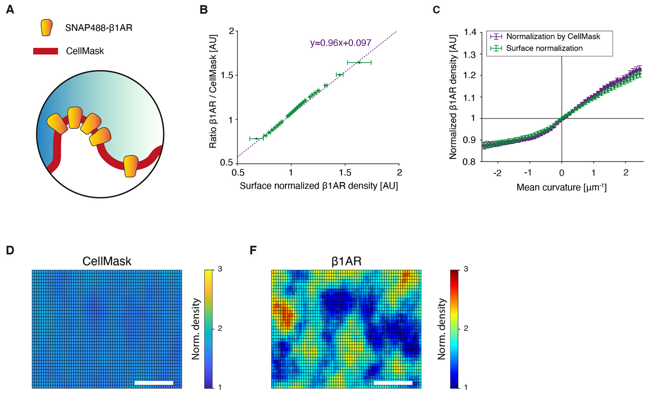
(a) Schematic of experimental approach. HEK293 cells express SNAP-β1AR and are labelled with SS488, while the membrane is labelled with CellMask DeepRed. (b) β1AR density normalized by recovered membrane surface area versus β1AR density normalized by CellMask intensity. The dashed purple line is a linear fit to the data. Data is shown as error-weighted bins with equal number of data points per bin. Error bars, s.e.m for y-axis and s.d. for x-axis. (c) Normalized β1AR density versus mean curvature. Recovery of normalized β1AR density by surface normalization (green) or by CellMask intensity (purple) results in the same density-curvature correlation. Data is binned using an error-weighted rolling average (0.1 ± 0.1 μm⁻¹) with error bars showing s.e.m. Data is from n = 7 cells from n = 1 experiment. (d-e) 2D projection of topography-corrected and normalized density of CellMask and β1AR for the same region at the PM. CellMask density is uniform at the PM (d), whereas β1AR forms domains (e). Scalebar, 500 nm.

Extended Data Fig. 7 |. Neither high-density nor low-density actin zones associate with domains of well-defined topography or mean curvature.

(a) Actin intensity at the plasma membrane overlaid with boundaries of high- and low-density zones of actin. Scale bar, 500 nm. (b) Density map of normalized β1AR overlaid with the actin boundaries from (a). Domain 1 in (a) and (b) indicates a low-actin-density region that contains both β1AR-enriched and -depleted domains. (c) Colocalization analysis of high- and low-density zones of actin with β1AR-enriched and -depleted domains. The colocalization percentages are compared to those of randomized actin zones. Quantitative correlations between high-/low-density actin regions and β1AR density patterns were either statistically nonsignificant or had low significance (P = 0.06 n.s., P = 0.03). P values are calculated by a two-sided paired t test. Data are the mean ± s.d. for n_C = 23, n_R = 2. (d) Membrane topography overlaid with the actin boundaries from (a). High- and low actin density zones are not preferentially colocalizing with membrane peaks or valleys. (e) Mean curvature overlaid with actin boundaries from (a). There is no preferential overlap of high- and low actin zones with positive or negative curvatures. Overlays are representative for n = 23 cells and n = 2 experiments.

Extended Data Fig. 8 |. Activation by agonist induces clathrin redistribution from receptor-depleted domains to both receptor-enriched and -depleted domains.

(a) Representative XY micrographs of SNAP-β1AR (magenta) and pmKate2-clathrin (green) and a merge in HEK293 cells. (b-c) XZ micrograph of β1AR, clathrin and a merge. Clathrin colocalizes with depleted domains of β1AR (b), but not with β1AR-enriched domains in the apo state (c). (d-f) XZ micrographs of events of β1AR internalization via clathrin-mediated endocytosis (indicated by arrows) after addition of ISO. These events are removed in our image analysis pipeline for recovering membrane topography and GPCR density. For (b-f) β1AR is imaged in 3D STED (magenta), clathrin in confocal (green) and a merge is shown. (g-h) 2D projection of normalized clathrin (g) and β1AR density (h) in the apo state. Arrows indicate regions of clathrin colocalizing with β1AR-depleted and not with β1AR-enriched domains. (i-j) 2D projection of normalized clathrin (i) and β1AR density (j) after activation by ISO. Arrows indicate regions of clathrin colocalizing both with β1AR-enriched and -depleted domains, however β1AR-enriched and -depleted domains do not always colocalize with clathrin (arrow with asterisk). (k) Colocalization analysis of high-density clathrin regions with β1AR-enriched and -depleted domains before and after activation by isoproterenol (ISO). The colocalization percentages are compared to randomized clathrin zones. Under basal conditions, β1AR and clathrin were anticorrelated (P = 0.01), while after activation with the agonist ISO, clathrin colocalization with GPCR-enriched domains was not statistically significant (P = 0.65). P values are calculated by a two-sided paired t test. Data are mean ± s.d. for n_C = 18, n_R = 3. Scalebar, (a) 1 μm, (b-f) 200 nm, (g-j) 500 nm.

Extended Data Fig. 9 |. Changes in membrane topography, curvature and β1AR density after cell flattening with an agarose pad.

Change in height (a), mean membrane curvature (b) and β1AR density (c) calculated by subtracting the values after flattening from the values before flattening (Fig. 3c,e,g and d,f,h). (d) Quantification of absolute change in height after flattening with an agarose pad from data in (a). The red line indicates the average change in membrane height of 14.5 nm. (e) Comparison of histograms of mean curvature of unperturbed (blue) and flattened (orange) for a single, representative HEK293 cell. After flattening the width of the histogram is smaller compared to the unperturbed cells. (f) Histograms of normalized β1AR density before (blue) and after (orange) flattening of the same cell as in (e). Normalized density of compressed cells shifts towards unity and the width of the histogram decreases. Data is representative for n = 10 cells in n = 5 replicates.

Extended Data Fig. 10 |. Domains of H-Ras, Piezo1 and EGFR at the PM of live cells.

2D projection of H-Ras density (a), overlay of H-Ras density on super-resolved topography map (b) and mean curvature map (c) of membrane topography shown in (b). H-Ras-enriched domains are formed at negative shallow curvature (see also Fig. 5d). (d-f) 2D projection of Piezo1 density (d), overlay of Piezo1 density on super-resolved topography map (e) and mean curvature map (f). Piezo1-enriched domains have high contrast and strongly couple to positive shallow curvature (see Fig. 5e). (g-i) 2D projection of EGFR density (g), overlay of EGFR density on super-resolved topography map (h) and mean curvature map (i). EGFR density variations couple to positive shallow curvature and are similar to those of β1AR and other studied GPCRs (see Supplementary Fig. 23). Black arrows indicate examples of H-Ras-, Piezo1- and EGFR-enriched domains. Scalebar (a,d,g), 500 nm.

Data availability

The structure of the inactive β1AR is available from the Protein Data Bank with accession code 2YCW. Source data are provided with this paper.

References

- 1.Pierce KL, Premont RT & Lefkowitz RJ Seven-transmembrane receptors. Nat. Rev. Mol. Cell Biol 3, 639–650 (2002). [DOI] [PubMed] [Google Scholar]
- 2.Weis WI & Kobilka BK The molecular bases of G protein-coupled receptor activation. Annu. Rev. Biochem 87, 879–919 (2018). [DOI] [PMC free article] [PubMed] [Google Scholar]
- 3.Wootten D, Christopoulos A, Marti-Solano M, Babu MM & Sexton PM Mechanisms of signalling and biased agonism in G protein-coupled receptors. Nat. Rev. Mol. Cell Biol 19, 638–653 (2018). [DOI] [PubMed] [Google Scholar]
- 4.Nikolaev VO et al. β2-Adrenergic receptor redistribution in heart failure changes cAMP compartmentation. Science 327, 1653–1657 (2010). [DOI] [PubMed] [Google Scholar]
- 5.Irannejad R. et al. Functional selectivity of GPCR-directed drug action through location bias. Nat. Chem. Biol 13, 799–806 (2017). [DOI] [PMC free article] [PubMed] [Google Scholar]
- 6.Briddon SJ, Kilpatrick LE & Hill SJ Studying GPCR pharmacology in membrane microdomains: fluorescence correlation spectroscopy comes of age. Trends Pharmacol. Sci 39, 158–174 (2018). [DOI] [PubMed] [Google Scholar]
- 7.Insel PA et al. Compartmentation of G-protein-coupled receptors and their signalling components in lipid rafts and caveolae. Biochem. Soc. Trans 33, 1131–4 (2005). [DOI] [PubMed] [Google Scholar]
- 8.Pontier SM et al. Cholesterol-dependent separation of the β2-adrenergic receptor from its partners determines signaling efficacy: insight into nanoscale organization of signal transduction. J. Biol. Chem 283, 24659–24672 (2008). [DOI] [PMC free article] [PubMed] [Google Scholar]
- 9.Lohse MJ & Hofmann KP Spatial and temporal aspects of signaling by G-protein-coupled receptors. Mol. Pharmacol 88, 572–578 (2015). [DOI] [PubMed] [Google Scholar]
- 10.Calebiro D & Sungkaworn T Single-molecule imaging of GPCR interactions. Trends Pharmacol. Sci 39, 109–122 (2018). [DOI] [PubMed] [Google Scholar]
- 11.Halls ML et al. Plasma membrane localization of the μ-opioid receptor controls spatiotemporal signaling. Sci. Signal 9, ra16 (2016). [DOI] [PubMed] [Google Scholar]
- 12.Sungkaworn T. et al. Single-molecule imaging reveals receptor-G protein interactions at cell surface hot spots. Nature 550, 543–547 (2017). [DOI] [PubMed] [Google Scholar]
- 13.Sezgin E, Levental I, Mayor S & Eggeling C The mystery of membrane organization: composition, regulation and roles of lipid rafts. Nat. Rev. Mol. Cell Biol 18, 361–374 (2017). [DOI] [PMC free article] [PubMed] [Google Scholar]
- 14.Annibale P & Lohse MJ Spatial heterogeneity in molecular brightness. Nat. Methods 17, 273–275 (2020). [DOI] [PubMed] [Google Scholar]
- 15.Adler J, Shevchuk AI, Novak P, Korchev YE & Parmryd I Plasma membrane topography and interpretation of single-particle tracks. Nat. Methods 7, 170–171 (2010). [DOI] [PubMed] [Google Scholar]
- 16.Eichel K & von Zastrow M Subcellular organization of GPCR signaling. Trends Pharmacol. Sci 39, 200–208 (2018). [DOI] [PMC free article] [PubMed] [Google Scholar]
- 17.Rosholm KR et al. Membrane curvature regulates ligand-specific membrane sorting of GPCRs in living cells. Nat. Chem. Biol 13, 724–729 (2017). [DOI] [PubMed] [Google Scholar]
- 18.Paszek MJ et al. Scanning angle interference microscopy reveals cell dynamics at the nanoscale. Nat. Methods 9, 825–827 (2012). [DOI] [PMC free article] [PubMed] [Google Scholar]
- 19.Elliott H. et al. Myosin II controls cellular branching morphogenesis and migration in three dimensions by minimizing cell-surface curvature. Nat. Cell Biol 17, 137–147 (2015). [DOI] [PMC free article] [PubMed] [Google Scholar]
- 20.Kabbani AM & Kelly CV The detection of nanoscale membrane bending with polarized localization microscopy. Biophys. J 113, 1782–1794 (2017). [DOI] [PMC free article] [PubMed] [Google Scholar]
- 21.van Rheenen J & Jalink K Agonist-induced PIP2 hydrolysis inhibits cortical actin dynamics: regulation at a global but not at a micrometer scale. Mol. Biol. Cell 13, 3257–3267 (2002). [DOI] [PMC free article] [PubMed] [Google Scholar]
- 22.Clack NG & Groves JT Many-particle tracking with nanometer resolution in three dimensions by reflection interference contrast microscopy. Langmuir 21, 6430–6435 (2005). [DOI] [PubMed] [Google Scholar]
- 23.Calebiro D. et al. Single-molecule analysis of fluorescently labeled G-protein-coupled receptors reveals complexes with distinct dynamics and organization. Proc. Natl Acad. Sci. USA 110, 743–748 (2013). [DOI] [PMC free article] [PubMed] [Google Scholar]
- 24.May S & Ben-Shaul A A molecular model for lipid-mediated interaction between proteins in membranes. Phys. Chem. Chem. Phys 2, 4494–4502 (2000). [Google Scholar]
- 25.Sperotto MM, May S & Baumgaertner A Modelling of proteins in membranes. Chem. Phys. Lipids 141, 2–29 (2006). [DOI] [PubMed] [Google Scholar]
- 26.Larsen JB et al. Membrane curvature enables N-Ras lipid anchor sorting to liquid-ordered membrane phases. Nat. Chem. Biol 11, 192–194 (2015). [DOI] [PubMed] [Google Scholar]
- 27.Larsen JB et al. Membrane curvature and lipid composition synergize to regulate N-Ras anchor recruitment. Biophys. J 113, 1269–1279 (2017). [DOI] [PMC free article] [PubMed] [Google Scholar]
- 28.Larsen JB et al. How membrane geometry regulates protein sorting independently of mean curvature. ACS Cent. Sci 6, 1159–1168 (2020). [DOI] [PMC free article] [PubMed] [Google Scholar]
- 29.Moukhametzianov R. et al. Two distinct conformations of helix 6 observed in antagonist-bound structures of a β1-adrenergic receptor. Proc. Natl Acad. Sci. USA 108, 8228–8232 (2011). [DOI] [PMC free article] [PubMed] [Google Scholar]
- 30.Lorent JH et al. Plasma membranes are asymmetric in lipid unsaturation, packing and protein shape. Nat. Chem. Biol 16, 644–652 (2020). [DOI] [PMC free article] [PubMed] [Google Scholar]
- 31.Marrink SJ et al. Computational modeling of realistic cell membranes. Chem. Rev 119, 6184–6226 (2019). [DOI] [PMC free article] [PubMed] [Google Scholar]
- 32.Latorraca NR, Venkatakrishnan AJ & Dror RO GPCR dynamics: structures in motion. Chem. Rev 117, 139–155 (2017). [DOI] [PubMed] [Google Scholar]
- 33.Zhao W. et al. Nanoscale manipulation of membrane curvature for probing endocytosis in live cells. Nat. Nanotechnol 12, 750–756 (2017). [DOI] [PMC free article] [PubMed] [Google Scholar]
- 34.McMahon HT & Gallop JL Membrane curvature and mechanisms of dynamic cell membrane remodelling. Nature 438, 590–596 (2005). [DOI] [PubMed] [Google Scholar]
- 35.Aimon S. et al. Membrane shape modulates transmembrane protein distribution. Dev. Cell 28, 212–218 (2014). [DOI] [PMC free article] [PubMed] [Google Scholar]
- 36.Brown MF Curvature forces in membrane lipid–protein interactions. Biochemistry 51, 9782–9795 (2012). [DOI] [PMC free article] [PubMed] [Google Scholar]
- 37.Hossein A & Deserno M Spontaneous curvature, differential stress, and bending modulus of asymmetric lipid membranes. Biophys. J 118, 624–642 (2020). [DOI] [PMC free article] [PubMed] [Google Scholar]
- 38.Soubias O, Teague WE Jr, Hines, K. G. & Gawrisch, K. Rhodopsin/lipid hydrophobic matching-rhodopsin oligomerization and function. Biophys. J 108, 1125–1132 (2015). [DOI] [PMC free article] [PubMed] [Google Scholar]
- 39.Joyce G, Robertson BD & Williams KJ A modified agar pad method for mycobacterial live-cell imaging. BMC Res. Notes 4, 73 (2011). [DOI] [PMC free article] [PubMed] [Google Scholar]
- 40.Bathe-Peters M et al. Visualization of β-adrenergic receptor dynamics and differential localization in cardiomyocytes. Proc. Natl Acad. Sci. USA 118, e2101119118 (2021). [DOI] [PMC free article] [PubMed] [Google Scholar]
- 41.Zhang Y et al. Cryo-EM structure of the activated GLP-1 receptor in complex with a G protein. Nature 546, 248–253 (2017). [DOI] [PMC free article] [PubMed] [Google Scholar]
- 42.Murthy SE, Dubin AE & Patapoutian A Piezos thrive under pressure: mechanically activated ion channels in health and disease. Nat. Rev. Mol. Cell Biol 18, 771–783 (2017). [DOI] [PubMed] [Google Scholar]
- 43.Zhou R, Han B, Xia C & Zhuang X Membrane-associated periodic skeleton is a signaling platform for RTK transactivation. Science 365, 929–934 (2019). [DOI] [PMC free article] [PubMed] [Google Scholar]
- 44.Antonny B Mechanisms of membrane curvature sensing. Annu. Rev. Biochem 80, 101–123 (2011). [DOI] [PubMed] [Google Scholar]
- 45.Iversen L, Mathiasen S, Larsen JB & Stamou D Membrane curvature bends the laws of physics and chemistry. Nat. Chem. Biol 11, 822–825 (2015). [DOI] [PubMed] [Google Scholar]
- 46.Bassereau P. et al. The 2018 biomembrane curvature and remodeling roadmap. J. Phys. D Appl. Phys 51, 343001 (2018). [DOI] [PMC free article] [PubMed] [Google Scholar]
- 47.Lingwood D & Simons K Lipid rafts as a membrane-organizing principle. Science 327, 46–50 (2010). [DOI] [PubMed] [Google Scholar]
- 48.Hatzakis NS et al. How curved membranes recruit amphipathic helices and protein anchoring motifs. Nat. Chem. Biol 5, 835–841 (2009). [DOI] [PubMed] [Google Scholar]
- 49.Huang W. et al. Structure of the neurotensin receptor 1 in complex with β-arrestin 1. Nature 579, 303–308 (2020). [DOI] [PMC free article] [PubMed] [Google Scholar]
- 50.Foerster F. et al. Targeting the actin cytoskeleton: selective antitumor action via trapping PKCε. Cell Death Dis. 5, e1398 (2014). [DOI] [PMC free article] [PubMed] [Google Scholar]
- 51.Roffay C et al. Passive coupling of membrane tension and cell volume during active response of cells to osmosis. Proc. Natl Acad. Sci. USA 118, e2103228118 (2021). [DOI] [PMC free article] [PubMed] [Google Scholar]
- 52.Zimmerberg J & Kozlov MM How proteins produce cellular membrane curvature. Nat. Rev. Mol. Cell Biol. 7, 9–19 (2006). [DOI] [PubMed] [Google Scholar]
- 53.Wolfenson H, Yang B & Sheetz M Steps in mechanotransduction pathways that control cell morphology. Annu. Rev. Physiol 81, 585–605 (2019). [DOI] [PMC free article] [PubMed] [Google Scholar]
- 54.Zimmerberg J & Gawrisch K The physical chemistry of biological membranes. Nat. Chem. Biol 2, 564–567 (2006). [DOI] [PubMed] [Google Scholar]
- 55.Staudt T et al. Far-field optical nanoscopy with reduced number of state transition cycles. Opt. Express 19, 5644–5657 (2011). [DOI] [PubMed] [Google Scholar]
- 56.Shelton E, Serwane F & Campas O Geometrical characterization of fluorescently labelled surfaces from noisy 3D microscopy data. J. Microsc 269, 259–268 (2018). [DOI] [PubMed] [Google Scholar]
- 57.Lohse MJ, Nuber S & Hoffmann C Fluorescence/bioluminescence resonance energy transfer techniques to study G-protein-coupled receptor activation and signaling. Pharmacol. Rev 64, 299–336 (2012). [DOI] [PubMed] [Google Scholar]
- 58.Lambert NA & Javitch JA CrossTalk opposing view: weighing the evidence for class A GPCR dimers, the jury is still out. J. Physiol 592, 2443–2445 (2014). [DOI] [PMC free article] [PubMed] [Google Scholar]
- 59.Barbotin A. et al. z-STED imaging and spectroscopy to investigate nanoscale membrane structure and dynamics. Biophys. J 118, 2448–2457 (2020). [DOI] [PMC free article] [PubMed] [Google Scholar]
- 60.Uline MJ & Szleifer I Mode specific elastic constants for the gel, liquid-ordered, and liquid-disordered phases of DPPC/DOPC/cholesterol model lipid bilayers. Faraday Discuss. 161, 177–191 (2013). [DOI] [PMC free article] [PubMed] [Google Scholar]
- 61.Keppler A et al. A general method for the covalent labeling of fusion proteins with small molecules in vivo. Nat. Biotechnol 21, 86–89 (2003). [DOI] [PubMed] [Google Scholar]
- 62.Sungkaworn T, Rieken F, Lohse MJ & Calebiro D High-resolution spatiotemporal analysis of receptor dynamics by single-molecule fluorescence microscopy. J. Vis. Exp 10.3791/51784 (2014). [DOI] [PMC free article] [PubMed] [Google Scholar]
- 63.Maiellaro I, Lohse MJ, Kittel RJ & Calebiro D Real-time monitoring of GPCR/cAMP signalling by FRET and single-molecule microscopy. Horm. Metab. Res 46, 827–832 (2014). [DOI] [PubMed] [Google Scholar]
- 64.Curtis A. The mechanism of adhesion of cell to glass: a study by Interference reflection microscopy. J. Cell Biol 20, 199–215 (1964). [DOI] [PMC free article] [PubMed] [Google Scholar]
- 65.Limozin L & Sengupta K Quantitative reflection interference contrast microscopy (RICM) in soft matter and cell adhesion. ChemPhysChem 10, 2752–2768 (2009). [DOI] [PubMed] [Google Scholar]
- 66.Barr VA & Bunnell SC Interference reflection microscopy. Curr. Protoc. Cell Biol 4, 4.23 (2009). [DOI] [PMC free article] [PubMed] [Google Scholar]
- 67.Kukulski W et al. Precise, correlated fluorescence microscopy and electron tomography of lowicryl sections using fluorescent fiducial markers. Methods Cell. Biol 111, 235–257 (2012). [DOI] [PubMed] [Google Scholar]
- 68.Biswas A, Alex A & Sinha B Mapping cell membrane fluctuations reveals their active regulation and transient heterogeneities. Biophys. J 113, 1768–1781 (2017). [DOI] [PMC free article] [PubMed] [Google Scholar]
- 69.Vicidomini G. et al. STED nanoscopy with time-gated detection: theoretical and experimental aspects. PLoS ONE 8, e54421 (2013). [DOI] [PMC free article] [PubMed] [Google Scholar]
- 70.Manders EMM, Verbeek FJ & Aten JA Measurement of co-localization of objects in dual-colour confocal images. J. Microsc 169, 375–382 (1993). [DOI] [PubMed] [Google Scholar]
Associated Data
This section collects any data citations, data availability statements, or supplementary materials included in this article.
Supplementary Materials
Data Availability Statement