Artificial Neural Networks for Short-Form Development of Psychometric Tests: A Study on Synthetic Populations Using Autoencoders

Abstract

Short-form development is an important topic in psychometric research, which requires researchers to face methodological choices at different steps. The statistical techniques traditionally used for shortening tests, which belong to the so-called exploratory model, make assumptions not always verified in psychological data. This article proposes a machine learning–based autonomous procedure for short-form development that combines explanatory and predictive techniques in an integrative approach. The study investigates the item-selection performance of two autoencoders: a particular type of artificial neural network that is comparable to principal component analysis. The procedure is tested on artificial data simulated from a factor-based population and is compared with existent computational approaches to develop short forms. Autoencoders require mild assumptions on data characteristics and provide a method to predict long-form items’ responses from the short form. Indeed, results show that they can help the researcher to develop a short form by automatically selecting a subset of items that better reconstruct the original item’s responses and that preserve the internal structure of the long-form.

Introduction

In recent years, short-form development has become a fundamental part of psychometric research. According to a search on PsycINFO reported by Leite et al. (2008), 46 articles were published from 2001 to 2006 that developed short forms. We performed a similar search on the same database for peer-reviewed journal articles published from 2017 to 2022 which resulted in 129 articles, highlighting the significant growth in short-form development and use in psychological contexts.

The increasing demand for shorter tests can be attributed to several factors. Long tests can be expensive and time-consuming to administer and often produce low-quality responses and high nonresponse rates (Galesic & Bosnjak, 2009). In addition, the need for shorter tests may reflect the growing trend toward more frequent use of longitudinal studies and multivariate approaches in psychological research (e.g., Lansford et al., 2022; Vatou, 2022).

Short-form development is frequent in various fields of psychology, such as Personality Psychology (e.g., García-Rubio et al., 2020; Markos & Kokkinos, 2017; Siefert et al., 2020), Clinical Psychology (e.g., Lee et al., 2020; Pietrabissa et al., 2020; Zurlo et al., 2017), and Educational Psychology (e.g., Coelho & Sousa, 2020; Lowe, 2021; Mariani et al., 2019).

Our search on PsycINFO also revealed that the prevalent techniques used for shortening tests are a mix of latent variable analysis techniques, item–total correlations, and Cronbach’s alpha (e.g., Bajcar & Babiak, 2022; Berry & Bell, 2021; Du et al., 2021).

Within this context, the aim is to develop a short form that maintains the characteristics of reliability and validity as similar as possible to the original long form. Indeed, as discussed by Leite et al. (2008), researchers typically investigate various types of validity evidence for the newly created short form: This evidence may relate to the short form’s internal validity or external validity, such as its correlations with the full form, other scales, or variables. However, as noted by Raborn et al. (2020), the focus often lies on maintaining the internal structure of the short form rather than preserving its external relationships with other variables. Traditional shortening methods present challenges in developing short forms that present satisfactory internal, as well as external validity. Researchers must choose an appropriate set of items from numerous combinations and assess the reliability and validity of the new form. This process can be very demanding in terms of time and resources, which may not always be available. Furthermore, the above-mentioned methods also rely on several assumptions, including the requirement that the relationships among variables are linear, thanks to the widespread use of Factor Analysis. While verifying this assumption can be difficult with psychological data, ignoring nonlinear relationships can result in misleading interpretations of results (Bauer, 2005; Belzak & Bauer, 2019) and inappropriate item selection.

From a more general perspective, the discussed methods traditionally used for short-form development, such as correlation or latent variables analysis techniques (e.g., exploratory and confirmatory factor analyses), can be reconducted to a statistical approach defined as “explanatory modelling” (Shmueli, 2011) or “data modelling culture” (Breiman, 2001). In this framework, researchers are interested in testing the hypothesized “true” relationship between variables and in studying their intercorrelations.

In recent years, various optimization algorithms linked to such an approach have been proposed to automate and optimize short-form development while reducing the validation steps. The optimization criteria proposed by these studies are mainly related to explained variance or the fit indices of Confirmatory Factor Analysis. Examples of these algorithms include the genetic algorithm (GA) proposed by Yarkoni (2010) and the ant colony optimization (ACO) algorithm proposed by Leite et al. (2008). These algorithms enable the optimization of multiple criteria, including internal and external validity, simultaneously.

However, in addition to exploratory modeling, the statistical approach called “predictive modeling” or “algorithmic modeling culture” can be also applied. This approach is used when the data generation process is unknown, and researchers aim to find an algorithm capable of recognizing patterns hidden in data and providing the best prediction for output values through input values of new observations. Although predictive modeling is less frequent in psychological research, it should be used when the primary objective is to predict entirely new observations that do not belong to the sample used for model construction (Yarkoni & Westfall, 2017).

Prediction and explanation are two different research goals that lead to different research processes and results. Integrating both explanatory and predictive views could improve research efficiency and facilitate the evaluation of model performance (Yarkoni & Westfall, 2017).

Despite predictive techniques being more frequent in psychometric research (Dolce et al., 2020; Edwards & Lowe, 2021; Orrù, Monaro, Conversano, Gemignani, & Sartori, 2020; Rao et al., 2022; Simeoli et al., 2021), they have been less applied to short-form development. However, we consider this approach a valuable alternative to traditional psychometric methods for shortening tests.

In line with the previous considerations, this contribution follows an integrative approach discussed by Hofman et al. (2021), which aims to estimate the true relationships among variables while considering their impact on predicting entirely new outcomes as accurately as possible.

In particular, the present study proposes a procedure to automatize the shortening process by integrating explanatory and predictive techniques. The proposed procedure uses a particular type of artificial neural network (ANN), the autoencoder, which is a dimensionality reduction technique comparable to principal component analysis (PCA). Autoencoders permit the integration of the explanatory and the predictive point of view in the same method: indeed, for its characteristics, it gives the possibility to predict the long-form pattern responses maintaining the interpretability of the data dimensions. Autoencoders have been widely applied in other scientific fields (e.g., Gokhale et al., 2022; Zhang & Dai, 2022) but are rarely used in the psychometric context. Despite this, we believe that their characteristics could help the researcher to select items with higher external validity, that is selecting items that better predict the entire pattern of responses of the original long-form. Furthermore, because of their relationship with other dimensionality reduction techniques, we hypothesize that the autoencoder also preserves the dimensionality of the original long form, and the internal validity of the short form (Casella et al., 2021).

In particular, this work aims to compare the item selection functioning of two different autoencoders: A linear autoencoder that for its characteristics is totally equivalent to PCA, and a multilayered non-linear autoencoder (NL-AE). The central idea of this study is to present an automatized procedure that sorts the items according to their importance for predicting long-form response patterns. The procedure aims to provide a guideline to the researcher for selecting items to include in the final short form.

The autoencoders are tested on artificial data generated from a factor-based population because of their diffusion in psychometric research. The different performance in item selection for short-form construction is evaluated considering the characteristics of the selected item (their relationship with the latent variable), the reconstruction error and the accuracy in reconstructing the item’s responses of the original long-form.

The results of the procedure are compared with two optimization algorithms for short-form development, the ACO and GA.

The article is organized as follows: First, we review more in detail the traditional techniques for shortening and their limits; then we discuss the machine learning approach for item selection and scale validation. At this point, we introduce our methods, the item-selection procedure and the way in which data are simulated. Next, we present the results of the procedure and the comparison with ACO and GA. Finally, we discuss the results and future directions.

Short-Form Development in Psychometric Research

Psychometric tests are typically shortened based on several criteria, such as statistic-driven strategies, content-related considerations, ad hoc strategies, or a combination of these (Kruyen et al., 2013; Levy, 1968).

Statistic-driven strategies are those predominantly based on classical test theory (CTT) and aim to maintain psychometric properties of the original scale (reliability and validity) approximately unaltered. This is achieved by considering items with the highest item–total correlation for a given construct or items with the highest factor loadings (in a factor analytic approach). In this context, there are several statistical techniques for investigating the internal structure of the original and shortened measure, such as PCA, exploratory factor analysis, and confirmatory factor analysis. Another common practice is to consider inter-item correlations or measures of internal consistency such as Cronbach’s alpha. Although reliability is lower when items are eliminated (because it depends on the number of items), the idea is to shorten the measure keeping an acceptable level of Alpha. As for the content-related strategy, experts evaluate items’ content and select those that best cover and represent the construct of interest (Kruyen et al., 2013).

Other approaches for shortening are those linked to item–response theory (IRT) and construct predictability. In the IRT, context items selected in constructing short forms are usually those with larger discrimination parameters or larger item-information functions than others (e.g., Colledani et al., 2018; Edelen & Reeve, 2007; Lau et al., 2021). The goal is to produce a latent variable that allows the highest measurement precision along the test.

The optimal shortening based on latent construct predictability is a short-form development approach proposed by Raykov et al. (2015), which aims to shorten psychometric tests without considerable loss in predictive power with respect to the underlying construct.

In this context, the term “predictive power” refers to the extent of relevant information about the latent variable contained in items, that is the degree to which items could be considered predictive of an underlying construct.

In particular, this method minimizes the loss in the instrument’s maximal reliability coefficient (ICP) implicated by measure shortening, removing iteratively items which least affect the ICP. This process is continued until a preset minimal threshold value of ICP is surpassed for the first time, or a prespecified length of the revised instrument is reached.

Despite its benefits, traditional short-form development hides some threats: for instance, as discussed by Smith et al. (2000), items that reflect a general construct show less correlation with those that define a more “subtly” defined construct, probably because they represent a small part of a more general construct. Therefore, not considering items with lower item–total correlation results in not considering some important aspects of the construct and, consequently, altering its meaning.

Furthermore, as mentioned above, statistics based on CTT can capture only linear relationships among items. Nevertheless, since relations met in the real world should be not always linear, these measures may not always be the appropriate methods of analysis.

Constructing a short form is a combinatorial problem with a very high number of possible solutions. In reality, few possible abbreviated combinations are considered, and this can lead to choosing nonoptimal solutions. In addition to this, the development of a short form requires the researcher to make decisions and intervene in the process: This increases the risk of erroneous decisions and biased instruments.

In recent years, several machine learning techniques have been proposed for shortening and scale development (see Raborn et al. (2020) and Gonzalez (2020) for a review and a comparison of these techniques). The applications of these methods in the psychometric context are briefly presented in the following section.

Machine Learning Techniques for Item Selection and Scale Validation

The selection of items to be included in a short form can be treated as a feature selection problem, a common task in machine learning, a subfield of artificial intelligence that includes many different computational operations, such as ANN and optimization algorithms. In recent years, these techniques have been applied in item selection and scale validation.

A study from Yarkoni (2010) applied GA to shortening personality inventories. GAs are inspired by natural evolution and are widely used for multi-objective optimization problems. This study validated the use of an algorithmic approach to personality measure shortening. In particular, the function optimized by the GA maximizes the amount of variance of the original long-form explained by the short-form and minimizes the number of items. So, the perfect solution is the short form with the least number of items and the highest amount of explained variance. The fitness function of this study had the form:

$$\begin{array}{c}\mathrm{Cost}=\mathrm{Ik}+\sum _{i=1}^{S}1-R_i^2\hfill \end{array}$$ (1)

where I is a fixed item cost, k is the number of items retained by the GA, s is the number of data dimensions (the subscales), and R²_i is the amount of variance in the ith subscale dimension that can be explained by a linear combination of individual item scores. The GA aims to find a solution that minimizes the fitness function. The parameter I determines the trade-off between brevity and explained variance, allowing the researcher to emphasize one over the other. A high value of I favors brevity, resulting in a relatively shorter measure even if it sacrifices some explained variance. Conversely, a low value of I prioritizes explained variance, leading to a measure with fewer items that still explains a substantial amount of variance.

Another study (Leite et al., 2008) proposes an ACO algorithm to select a subset of items that could optimize the parameter of a structural equation model. ACOs are multiagent systems based on the foraging behavior of real ants who can find the shortest path from their colony to a food source by following chemical feedback, called pheromone, repeatedly left on the ground by other ants (Dorigo et al., 2006). In particular, the study of Leite and colleagues (2008) implements the ACO algorithm to obtain a subset of items that have the same internal structure as the original test and a maximal relationship with an external variable. In particular, Leite et al. (2008) used this algorithm to select items that could optimize simultaneously the model fit (in particular, comparative fit index [CFI], Tucker–Lewis index [TLI], and root mean square error of approximation [RMSEA] measures) and a relationship with an external variable.

Another approach proposed by Dolce et al. (2020) also considers the internal structure and the relationship with external criteria but uses ANN for scale construction and validation. In this study, authors have proposed a procedure for item selection that considers both the exploratory data analysis for investigating the dimensional structure and the ANN for predicting the psychopathological diagnosis of clinical subjects (a classification problem).

The explanatory view permits theoretical insights into the characteristics of the selected items and their conformity with the theoretical framework of reference. At the same time, the use of the ANN permits the selection of items more predictive of the external criteria (the psychopathological diagnosis).

In line with such an approach, this study introduces a short-form development procedure that uses a particular type of ANN, the autoencoders, which could help in constructing short forms that better predict the long-form response patterns. Differently from other discussed techniques, autoencoders do not optimize fit indices related to an explanatory approach, but they could learn the most important relationships in data for their architecture and for its characteristics, similar to traditional dimensionality reduction methods used in psychometric research.

Method

Autoencoders

Autoencoders are ANNs first introduced by LeCun (1987) and later developed by Baldi and Hornik (1989), widely used in several scientific fields for customer segmentation, image recognition, and dimensionality reduction problems (Alkhayrat et al., 2020; Hammouche et al., 2022).

In general, a dimensionality reduction technique produces an approximation ${\hat{x}}_j$ to the original variable x_j, where j is a generic variable of the p total variables, and x is a single observation. This approximation results from the combination of two functions, f and g:

$$\begin{array}{c}{x}_j={\hat{x}}_j+{ϵ}_j=g\left(f\left(x_j\right)\right)+{ϵ}_j,j=1,2,\dots ,p\hfill \end{array}$$ (2)

The projection function f : R_p→R_z projects the original high-dimensional data x_j onto a z-dimensional subspace with lower dimensionality, while the expansion function g : R_z→R_p defines a mapping from the z-dimensional space back into the original high-dimensional space with a residue ϵ_j. The dimensionality reduction problem is resolved through the determination of functions f and g.

The autoencoder performs dimensionality reduction thanks to its particular architecture represented in Figure 1.

Figure 1.

Autoencoder’s Typical Architecture

In particular, an autoencoder has the same inputs as target outputs and a smaller central layer, usually called the “bottleneck layer.” This network aims to reconstruct the input vectors as better as possible, usually minimizing a reconstruction error function of the form:

$$\begin{array}{c}\mathrm{MSE}=E[x_j-g{\left(f\left(x_j\right)\right)}^2]\hfill \end{array}$$ (3)

Perfect reconstruction of inputs is not possible because the bottleneck layer is smaller than the input/output layers, but the idea is that this layer encodes the most relevant information for reconstructing data. So, the dimensionality reduction is achieved in the bottleneck layer.

An autoencoder can be logically divided into two parts: an encoder and a decoder. The encoder compresses data points into a lower dimensional latent space (the bottleneck layer), while the decoder expands data back from the bottleneck layer to the original high-dimensional space. In this case, the encoder can be seen as the projection function g mentioned above, while the decoder is the expansion function f.

In general, the encoder and the decoder can use nonlinear activation functions (e.g., sigmoid, tanh), whereas, when the autoencoder is used for dimensionality reduction, the bottleneck layer has usually linear activations.

Considering these characteristics, autoencoders show a similarity with another famous dimensionality reduction technique: the PCA.

PCA aims to reduce a large set of variables preserving as much information as possible (Hotelling, 1933). This is possible by creating new variables, the principal components, which are a synthesis of the original variables.

PCA handles the dimensionality reduction problem via the eigenvalue decomposition, which is a particular case of the more general singular value decomposition. The starting point is the data variance–covariance matrix and PCA is usually solved by extracting the eigenvalues of this matrix. Because of their proprieties, the sum of the eigenvalues is equal to the total variance of data and the single eigenvalue is a measure of the principal component’s explained variance. PCA can be also viewed as a minimization problem: indeed, its goal is to minimize the error in reconstructing observations as a linear combination of weighted principal components (Jolliffe, 2003).

It was shown that an autoencoder with a single linear hidden layer with z units, performs a projection onto the z-dimensional subspace which is spanned by the first z principal components of the data (Baldi & Hornik, 1989; Bourlard & Kamp, 1988). Thus, the vectors of weights which lead into the bottleneck layer’s units form a basis set which spans the principal subspace. In this case, both PCA and autoencoders perform a linear dimensionality reduction and are minimizing the same reconstruction error function (Bishop & Nasrabadi, 2006). However, the nodes of the bottleneck layer are not exactly the principal components of data: indeed, the principal components are uncorrelated and sorted in order of relevance. These characteristics made the PCA solution more interpretable than the autoencoder solution. However, the autoencoder is not limited to linear transformations (Kramer, 1991); therefore, it can learn more complicated relations between inputs and bottleneck units.

Recently, authors have proposed a type of autoencoder (PCA-autoencoder [PCA-AE]) that makes explicit the PCA properties (Ladjal et al., 2019; Pham et al., 2020). Indeed, when used with a single linear hidden layer, this autoencoder is totally equivalent to PCA and its internal nodes are exactly the principal components of data (Casella et al., 2022).

This study aims to investigate the behavior of a NL-AE and a PCA-AE in item selection for short-form development. The item selection procedure will be presented in detail in the following section.

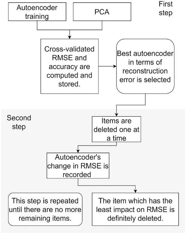
Item Selection Procedure

The item selection procedure is summarized in Figure 2.

Figure 2.

Item Selection Procedure

Note. PCA = principal component analysis; RMSE = root mean squared error.

In the first step, the autoencoder is trained on the long form. Fivefold cross-validation is performed to select the autoencoder with the lower root mean squared error (RMSE). In particular, we considered the RMSE computed on the validation fold to select the autoencoder which best predicts the original long form. RMSE is computed as follows:

$$\begin{array}{c}\mathrm{RMSE}(x_{\mathrm{ij}},{\hat{x}}_{\mathrm{ij}})=\sqrt{\frac{1}{n}\sum _{i=1}^n\left(\frac{\sum _{j=0}^p{(x_{\mathrm{ij}}-{\hat{x}}_{\mathrm{ij}})}^2}{p}\right)},\begin{array}{c}i=1,2,\dots ,n;\hfill \\ \multicolumn{1}{c}{j=1,2,\dots ,p}\end{array}\hfill \end{array}$$ (4)

where n is the number of subjects and p is the number of inputs.

A PCA is also performed on each training fold.

We computed two metrics to evaluate and compare PCA and autoencoder performances: RMSE and accuracy. Because it is not possible to predict test data from principal components, the cross-validated RMSE and the accuracy are computed on the training set both for autoencoders and PCA, to have comparable measures. More specifically, accuracy was computed as the proportion of correct predictions on the total number of predictions:

$$\begin{array}{c}\mathrm{Accuracy}=\frac{1}{n}\left(\sum _{i=1}^n\left(\frac{\sum _{j=1}^{p}H(x_{\mathrm{ij}},{\hat{x}}_{\mathrm{ij}})}{p}\right)\right),H(x_{\mathrm{ij}},{\hat{x}}_{\mathrm{ij}})=\{\begin{array}{c}0,\mathrm{if}{x}_{\mathrm{ij}}\ne {\hat{x}}_{\mathrm{ij}}\hfill \\ \multicolumn{1}{c}{1,\mathrm{if}{x}_{\mathrm{ij}}={\hat{x}}_{\mathrm{ij}}}\end{array}\hfill \end{array}$$ (5)

where n is the number of subjects, p is the number of inputs and $H(x_{\mathrm{ij}},{\hat{x}}_{\mathrm{ij}})$ is a binary function that can assume only two values.

The second step is implemented more specifically the item selection procedure.

To understand which items were the most important in reconstructing the long form, we assessed the variation in the RMSE of the autoencoder by sequentially removing items. This approach, called Improved stepwise selection 1 (Olden et al., 2004; Simeoli et al., 2021), reduces the computational effort.

As proposed by Dolce et al. (2020), it is alternatively possible to consider n random combination of features, to select items in common across all the “best” solutions in terms of prediction accuracy, to fix the selected items and then again sample from the set of the remaining items, until the algorithm figured out which set of items achieves the best prediction accuracy. This procedure, however, requires more computational effort.

In this work, starting from the entire set of x₁, x₂, _{. . .}, x_p items, and considering the whole dataset, we recorded the change in RMSE after the removal of every item, one at a time. Once the item with the lesser impact on the RMSE was identified, it was permanently removed (i.e., the input of the neural network which encoded this item was set to 0). The procedure had p steps; in other words, it stopped when the number of remaining p items was exhausted.

We speculate that the change in RMSE for each removed item is an indication of its relative importance: In particular, the idea is that when an item is not very important in reconstructing the long form, after its elimination the reconstruction error has a minimal increase. Indeed, at this point, it was possible to define an order of importance where the last items selected by the procedure were those that best reconstruct the long form.

For each item elimination step, we computed also autoencoder accuracy.

Finally, we performed PCA on the last items preserved by the procedure to investigate the internal structure of the resulting short form. The number of items to retain can be selected following two strategies: by setting a prechosen number of items to preserve or by setting a threshold on the evaluation metrics.

Since indicators have different degrees of importance, our hypothesis was that the trained autoencoders could be able to remove items in order of relevance and preserve items with the highest factor loadings (items that better reflect the underlying construct) for each latent variable until the last steps of the procedure.

Simulation Design and Data Generation

Data are simulated considering the theoretical path model shown in Figure 3, using R software and the LAVAAN package (Rosseel, 2012).

Figure 3.

Path Model for Data Generation

The model has a three-dimensional structure and nine indicators for each dimension (27 total indicators). The factor loadings assume three different values: 0.3, 0.6, and 0.8.

The number of dimensions and indicators is arbitrarily chosen. Indeed, the goal was to simulate a multidimensional structure and different factor loadings levels.

Since we want to test the procedure avoiding the risk of intervenient variables and varying only some design factors, indicators have no measurement error and assume categorical values in a range that goes from 1 to 5 (as a traditional Likert-type scale). Latent variables have variance set to 1, they are uncorrelated and normally distributed.

The simulation study considers four different sample sizes: 200, 500, 700, and 1,000.

To obtain stable average outcomes for analyses, we conducted 500 replications for each sample size, resulting in the generation of 4*500 = 2,000 datasets.

The average fit indices of confirmatory factor analysis performed on all datasets are optimal (CFI = 1.00, TLI = 1.00, RMSEA = 0.00). It is worth noting that the model is not just-identified (saturated) since its degrees of freedom are >0, and that our primary objective is not to validate the model, but to verify that the data dimensionality is preserved.

Indeed, the hypothesis is that the item selection procedure converges to an ideal solution that preserves the items with higher factor loadings for each simulated factor until the last steps of the procedure.

PCA-AE’s Architecture

This study considered a PCA-AE which had 27 inputs, three linear hidden neurons, and 27 outputs. This architecture aimed to ensure the equivalence between PCA and PCA-AE. Since the PCA is a linear transformation, we considered a neural network with one linear hidden layer and three nodes, as the number of simulated dimensions. In this case, we considered a single hidden layer because stacking multiple linear layers is redundant: Indeed, all the consecutive linear layers after the first are its linear transformation, so n linear layers can be replaced by a single linear layer.

Consequently, in PCA-AE used for this study, the encoder was the set of weights between the input layer and the bottleneck layer. In the same way, the decoder was the set of weights between the bottleneck layer and the outputs.

The PCA-AE has a particular training procedure, summarized in Figure 4, which ensures that the internal nodes of this autoencoder are orthogonal and ordered by explained variance.

Figure 4.

PCA-AE Training Procedure

Note. PCA-AE = principal component analysis-autoencoder.

In the first step, an autoencoder with only one internal node is trained and its weights are fixed. At this point, another internal neuron is added and the set of weights between the inputs and this second internal node is trained and fixed. The decoder of the previous step is discarded and a new one is trained from scratch at each step. This procedure continues until the required number of internal nodes is reached.

The loss function of PCA-AE had two parts: A mean squared error reconstruction error term and a covariance loss term which encourages the latent space to be orthogonal (for a detailed description of this autoencoder, see Pham et al. (2020) and Ladjal et al. (2019)). Weight initialization was from the uniform distribution suggested by Glorot and Bengio (2010), and the seed for weights initialization changed every 10 datasets to avoid the risk of biased results. The Adaptive moment estimation (Adam) learning algorithm was used to update the iterative network weights based on the training data (Kingma & Ba, 2015), and the learning rate was set at 0.005. Early stopping was implemented, so when the RMSE on the validation fold did not decrease for 40 epochs, training stopped. The correlation between nodes and principal components was computed for each dataset. Since both PCA and PCA-AE produced a continuous output, reconstructed scores are rounded before computing performance metrics.

NL-AE’s Architecture

For the second study, datasets were preprocessed by one-hot encoding: this data transformation technique is applied to categorical variables and creates a new binary feature for each possible category as shown in Figure 5.

Figure 5.

One-Hot Encoding Transformation of Original Item Responses

NL-AE used in this study had the architecture shown in Figure 1. Input layers and output layers had a size of 135 (27 × 5); the five hidden layers had sizes of 90, 40, 15, 40, and 90.

Hidden layers and the output layer had sigmoid activation functions, except for the bottleneck layer which had linear activation function.

The sigmoid activation function used for the encoding and decoding layers and for the output layer maps any input to an output ranging from 0 to 1 and is mostly used for binary classification. It has the form:

$$\begin{array}{c}\sigma \left(z\right)=\frac{1}{1+e^{-z}}\hfill \end{array}$$ (6)

where z is the net input of an artificial neuron defined as:

$$\begin{array}{c}z=\sum _j{w}_j{x}_j+b\hfill \end{array}$$ (7)

where w_j indicates the weights of the previous layer, x_j are the inputs received by the neuron and b represent bias.

For the training, we use a binary cross-entropy loss function to calculate the model error. The learning rate is set to 0.001. Early stopping is implemented so the autoencoder’s training stops after 20 epochs in which the loss function does not decrease. Weight initialization is from the uniform distribution and the seed for weights initialization changes every 10 datasets. For the item selection procedure, when an item is removed, all the five neurons which encode this item are set to 0, whereas to compute performance metrics, the data are rescaled to the original 1 to 5 range.

Data Analysis and Results

PCA-AE and PCA training accuracy and RMSE are, on average, very similar (RMSE_PCA = 0.817, RMSE_PCA-AE = 0.817, Accuracy_PCA= 49.08%, Accuracy_PCA-AE = 48.95%). PCA-AE performance metrics are very similar also across all sample sizes as shown in Figure 6.

Figure 6.

PCA and PCA-AE Average RMSE (A) and Accuracy (B) for Each Simulated Sample Size

Note. PCA = principal component analysis; PCA-AE = principal component analysis-autoencoder; RMSE = root mean squared error.

Furthermore, PCA-AE internal nodes and principal components have a strong correlation, as reported in Table 1.

Table 1.

Correlations Among PCA-AE Internal Node Activations and Principal Components

Principal components	First node	Second node	Third node
First PC	0.96 ± 0.02	0.09 ± 0.04	0.01 ± 0.002
Second PC	0.09 ± 0.04	0.89 ± 0.04	0.22 ± 0.06
Third PC	0.02 ± 0.004	0.21 ± 0.07	0.92 ± 0.03

Note. The table reports the average correlations considering all replications and all sample sizes. The highest correlation values are highlighted in bold. PCA-AE = principal component analysis-autoencoder.

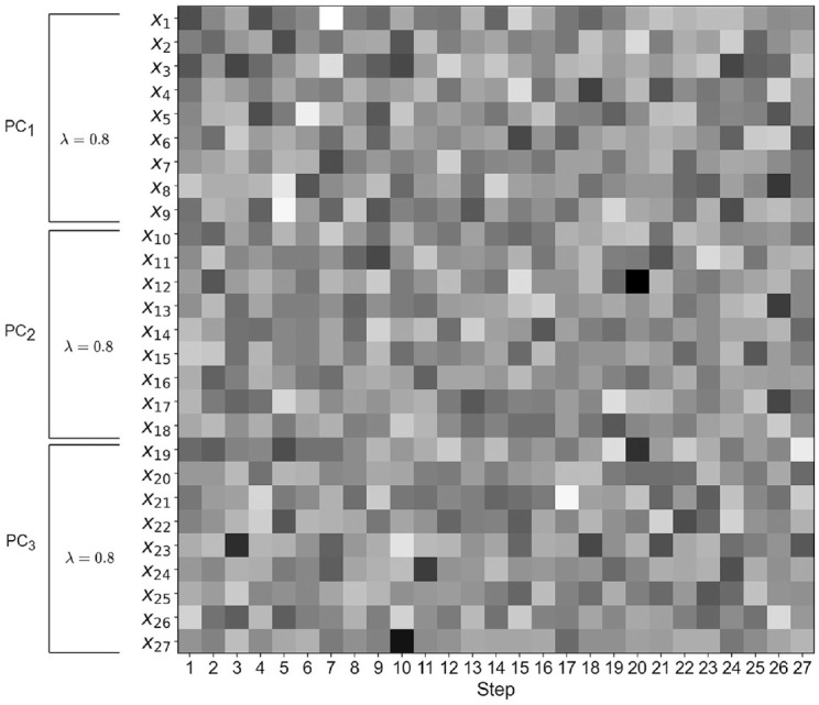
Figure 7 shows the results of the item selection procedure: In particular, for each sample size, it shows with shades of gray how many times on the 500 replications a single item is removed by the iterative selection procedure. We compare this result with a “control” model where all factor loadings are set to 0.8. For this model, all solutions are equivalent, so the selected items vary at each replication, and, on average, it could not be possible to see a “trend” in the elimination order (see Figure 8).

Figure 7.

PCA-AE’s Item Selection Procedure Results for Each Simulated Sample Size

Note. PCA-AE = principal component analysis-autoencoder.

Figure 8.

PCA-AE’s Item Selection Procedure Results on a Control Model

Note. The figure shows results for all replications and sample sizes. The control model has all factor loadings equal to 0.8

Note. PCA-AE = principal component analysis-autoencoder.

Concerning the model with different factor loadings, it is possible to identify a pattern where the most removed items follow the same order in all replications and sample sizes. Indeed, in the first nine iterations, the most selected items are those with a factor loading of 0.3, whereas in subsequent iterations, the removed items are those with loadings equal to 0.6. Only in the last iterations, items with factor loading equal to 0.8 are removed. However, the PCA-AE pattern in item selection is fuzzier when the sample size is 200 (see Figure 7). Despite this, the first items removed by the procedure are still the items with the lowest factor loading.

The autoencoder’s RMSE and accuracy computed at each item elimination step are reported in Figure 9. The RMSE shows a rapid increase after the first nine iterations, when the most important variables begin to be discarded. RMSE and Accuracy are similar for each considered sample size, except when N = 200: In this case, RMSE is lower, and accuracy is higher.

Figure 9.

PCA-AE RMSE (A) and Accuracy (B) for Each Step of the Item Selection Procedure

Note. PCA-AE = principal component analysis-autoencoder.

At this point, we performed PCA on the last nine items preserved by the procedure for each replication.

Table 2 reports the average proportion of the explained variation and the average eigenvalues of the first five PCs: They are higher for the first three components (in particular, the eigenvalues are >1) and very low for subsequent components. So, the PCA-AE preserves the original measure’s dimensionality and is equivalent to PCA in terms of accuracy and reconstruction error.

Table 2.

Average Proportion of Explained Variance and Eigenvalues of PCA-AE Short-Form Solutions

Sample size	First PC	Second PC	Third PC	Fourth PC	Fifth PC
200	0.27 (2.43)	0.21 (1.96)	0.17 (1.58)	0.09 (0.79)	0.07 (0.64)
500	0.28 (2.53)	0.23 (2.08)	0.17 (1.53)	0.07 (0.68)	0.07 (0.60)
700	0.28 (2.39)	0.24 (2.14)	0.18 (1.88)	0.07 (0.62)	0.05 (0.49)
1,000	0.28 (2.52)	0.24 (2.16)	0.18 (1.72)	0.07 (0.62)	0.05 (0.50)

Note. The table reports results for the first five principal components. Bold values indicate the principal components preserved from PCA-AE short-form solutions. PCA-AE = principal component analysis-autoencoder.

Concerning the NL-AE results, the average training accuracy computed on all datasets is higher for NL-AE than PCA-AE (Accuracy_PCA-AE= 48.95%, Accuracy_NL-AE = 59.18%). However, also RMSE is, on average, slightly higher for NL-AE (RMSE_PCA-AE = 0.817, RMSE_NL-AE = 0.854). Nevertheless, if we do not consider datasets with a sample size of 200, the average RMSE is about the same for NL-AE and PCA-AE (see Figure 10).

Figure 10.

NL-AE and PCA-AE Average RMSE (A) and Accuracy (B) for Each Simulated Sample Size

Note. NL-AE = non-linear autoencoder; PCA-AE = principal component analysis-autoencoder; RMSE = root mean squared error.

Figure 11 shows the results of the item selection procedure: Also in this case, at the first iterations, the predominantly selected items are those with a factor loading of 0.3 whereas the most preserved items are those with loadings equal to 0.8. However, as can be seen in the figure, this autoencoder tends to remove items with loadings of 0.6 throughout the iterative procedure and therefore has a fuzzier pattern in the intermediate steps. Also for this autoencoder, when the sample size is equal to 200, it is not possible to see a definite elimination trend, but the items with the highest factor loading are preserved until the end of the procedure.

Figure 11.

NL-AE’s Item Selection Procedure Results for Each Simulated Sample Size

Note. NL-AE = non-linear autoencoder.

Results of the item selection procedure are compared with results on a control model shown in Figure 12.

Figure 12.

NL-AE’s Item Selection Procedure Results on a Control Model

Note. The figure shows the results for all replications and sample sizes. The control model has all factor loadings equal to 0.8. NL-AE = non-linear autoencoder.

The autoencoder’s average RMSE and accuracy for different sample sizes at each item elimination step are reported in Figure 13. Both RMSE and accuracy show a similar trend: They are nearly stable until the last steps when the most important items are removed. This result could reflect the robustness of autoencoders (and ANNs as well), which are able to reconstruct observations with relatively high accuracy, also in case of noisy or deteriorated inputs. However, the performance metrics get worse with a sample size of 200.

Figure 13.

NL-AE RMSE (A) and Accuracy (B) for Each Step of the Item Selection Procedure

Note. NL-AE = non-linear autoencoder; RMSE = root mean squared error.

Table 3 reports the average PCA results for the last nine preserved items: The explained variance and the eigenvalues are higher for the first three components and lower for subsequent components. So, the NL-AE preserves the dimensionality of the original measure.

Table 3.

Average Proportion of Explained Variance and Eigenvalues of NL-AE Short-Form Solutions

Sample size	First PC	Second PC	Third PC	Fourth PC	Fifth PC
200	0.26 (2.36)	0.22 (1.99)	0.18 (1.64)	0.08 (0.77)	0.07 (0.63)
500	0.26 (2.35)	0.23 (2.09)	0.20 (1.85)	0.07 (0.65)	0.06 (0.56)
700	0.26 (2.39)	0.23 (2.14)	0.21 (1.89)	0.07 (0.62)	0.05 (0.49)
1,000	0.26 (2.34)	0.23 (2.15)	0.21 (1.88)	0.07 (0.64)	0.05 (0.50)

Note. The table reports results for the first five principal components. Bold values indicate the principal components preserved from NL-AE short-form solutions. NL-AE = non-linear autoencoder.

Furthermore, the total amount of explained variance of the first three components is, on average, very similar for PCA-AE and NL-AE solutions as shown in Table 4.

Table 4.

Cumulative Explained Variance by the First Three Components of PCA-AE and NL-AE Short-Form Solutions

Sample size	PCA-AE	NL-AE
200	0.65	0.66
500	0.68	0.69
700	0.70	0.70
1,000	0.70	0.70

Note. The table reports the average value computed on all 500 replications. PCA-AE = principal component analysis-autoencoder; NL-AE = non-linear autoencoder.

This result suggests that the short-form solutions of PCA-AE and NL-AE are nearly equivalent in terms of internal structure.

Comparison With Optimization Algorithms for Short-Form Development

To compare the performance of different approaches in developing short forms of psychometric tests, we used two optimization algorithms, the ACO and the GA, and compared their performance with PCA-AE and NL-AE.

The ACO and GA were, respectively, implemented using the R package “ShortForm” proposed by Raborn and Leite (2018) and “GAbbreviate” proposed by Scrucca and Sahdra (2016).

The values for tuning parameters are the same as proposed by Raborn et al. (2020). The parameters not reported in this study were set to default values. We selected 100 random replications of the 500 total datasets considering a sample size of 500. We chose this sample size to have similar conditions to the above-mentioned study.

We set the ACO and GA algorithms to retain three items for each simulated dimension, resulting in a short form of nine items for these methods.

For the NL-AE and PCA-AE, given that there is no a priori indication about the number of items to retain or their specific relationships with latent factors, we selected the last nine items preserved by the item selection procedure presented in this study.

The average fit indices of the confirmatory factor analysis performed on all the final short-form solutions are optimal for all tested algorithms (CFI = 1.00, TLI = 1.00, RMSEA = 0.00). This finding is particularly interesting for the PCA-AE and even more for the NL-AE cases. In fact, for the PCA-AE, we opted to use three central nodes to maintain the original three-dimensional structure, taking advantage of the similarities between PCA and PCA-AE. For the NL-AE, on the contrary, we do not have a direct comparison between nodes and principal components like we did for PCA-AE. Nevertheless, our results show that also in this case all factors are retained and well represented in final short-form solutions.

It is worth noting that these results can be influenced by the way in which data are simulated. In our study, the simulated datasets had a perfect factorial structure, which explains why all algorithms achieved optimal solutions in terms of fit indices. Indeed, the starting fit indices were already perfect, as our goal was to investigate the quality of emergent solutions in terms of their dimensionality and preserved relationships among inputs and factors.

Figure 14 reports for each dimension how many times each item is selected by the algorithms. PCA-AE and NL-AE converged to very similar solutions, in which the most selected items are those with the highest factor loadings. GA and ACO solutions present a less clear pattern in selecting items, with a homogeneous sampling across all items.

Figure 14.

Frequency of Choice of Each Item for the Compared Shortening Methods

Note. The figure shows, for each one of the three simulated components and considering 100 replications, how many times a single item is chosen by the four different shortening methods. The sample size is 500. ACO = ant colony optimization; GA = genetic algorithm; NL-AE = non-linear autoencoder; PCA-AE = principal component analysis-autoencoder.

General Discussion

In this study, we propose an automatized procedure for short-form development and investigate the differences between a linear PCA-AE and a multilayered NL-AE for item selection in terms of reconstruction error and accuracy.

Results show that both autoencoders preserve the dimensionality of the original measure and preserve items with greater loadings until the last steps. An important consideration is that the autoencoders do not have any a priori knowledge of the factorial structure of the data or indication on the number items to preserve. The solution emerges from the procedure, by only taking into account the reconstruction error between the input (the short form) and the output (the long form to be reconstructed) using the autoencoder trained on the long form. Indeed, autoencoders do not optimize fit indices or factor analysis parameters: This could be particularly relevant in real scenarios where the assumptions postulated by factor analysis are violated or relationships among variables are not linear.

However, the proposed autoencoders have different behaviors: PCA-AE is totally equivalent to PCA in terms of reconstruction error and accuracy, whereas the NL-AE has about the same reconstruction error, but higher accuracy. This is unsurprising since the NL-AE has a greater representational power (a greater number of layers and hidden neurons, and can model nonlinear relationships), despite the fact that its internal nodes can’t be reconducted to the principal components. In this case, the accuracy is higher but the solution is less interpretable.

However, the correlations between PCA-AE internal nodes and principal components make PCA-AE more interpretable. PCA-AE is also more precise than NL-AE in recognizing the order of importance of items when the sample size is large enough. However, for a sample size of 200, the performances of both autoencoders in item selection are poor. This might be due to a general characteristic of machine learning methods which work best with a large amount of data for training.

We also compared our procedure with two optimization algorithms, the ACO and GA. Although it is possible to compare the final short forms of all methods in terms of fit indices and items more frequently selected on the total replications, it is not possible to evaluate the accuracy and reconstruction error between the short form developed by ACO and GA and the original long-form responses, because those metrics derive from the proposed approach, which gives the possibility to train the autoencoder on the long form and evaluate the accuracy of a short form by using it to reconstruct the long-form responses.

The results of the comparison show that the various algorithms produce distinct solutions, all of them having an optimal fit. However, our approach tends to select items with the highest factor loadings. Indeed, the best solution, in our case, is the solution that preserves the items with the highest loadings, as they are strongly correlated with the factor, and our goal was to test whether the autoencoder was able to converge to that solution.

Data used in this study are simulated assuming linear relationships among items because we want to test the autoencoders in a condition that is comparable with other dimensionality reduction methods such as PCA, and we demonstrate that the autoencoders’ and PCA reconstruction error is about the same. Starting from this point, future research will investigate the performances of NL-AEs in selecting items on simulated data with nonlinear relationships and on real data.

It should be noted that the proposed procedure differs from other optimization techniques as it provides the researcher, aiming to shortening a test, with a ranking of item importance for reconstructing the long form, rather than a final short form.

The final shorter form, that is, the number of items to retain, can be determined by the researcher based on the autoencoder’s solution, allowing the researcher to take into account also additional content-related elements of the items.

As said, in this study, one of the evaluation metrics used is predictive accuracy: since PCA, per se, cannot predict test data from new observations, accuracy is computed on the training set both for autoencoders and PCA. In this sense, accuracy can be interpreted as “reconstruction” accuracy, rather than predictive accuracy. Nevertheless, autoencoders are predictive and generative methods, so they can reconstruct any new observations. This characteristic gives us the possibility to investigate an explanatory and a predictive point of view with a single method.

As an additional point of discussion, it is worth noting that, in this work, PCA is used to investigate the data internal structure. This choice is due to several reasons. First, PCA is frequently used in psychometric research for investigating test dimensionality, and famous psychological analysis software often used in psychology has PCA as the default method for dimensionality reduction (e.g., SPSS). Second, the relationship between PCA and autoencoders is well-known and investigated in previous research (Casella, 2022; Plaut, 2018).

However, we are aware of the limitation of this choice, since PCA is a mathematical transformation of data and not a latent variable detection technique. For some purposes, such as creating an index variable from various indicators, PCA could be a useful technique, but when the research goal is to validate psychological scales, researchers are interested in testing latent variables, and not just in reducing a large number of variables to fewer indices. In this context, latent variable techniques such as factor analysis may be more appropriate (e.g., Borsboom, 2006).

Considering this, future research will take into consideration variational autoencoders (VAE) (Kingma & Welling, 2014; Urban & Bauer, 2021), which are a particular type of autoencoders that encourage the latent space to follow a predefined distribution (e.g., normal distribution). This is achieved by modifying the autoencoder loss function by adding a regularization term, which ensures the regularity of the latent space and the correct approximation to the chosen conditional distribution. For its characteristics, VAE maps similar inputs closer into the latent space. So, the trained latent space has a metric which reflects the original differences in input vectors, in a sort of scaling of input vectors.

These characteristics allow for greater interpretability of latent space and a more direct comparison to latent variable analysis techniques.

In conclusion, we believe that integrating machine learning techniques can help overcoming the limits of traditional psychometric methods used for dimensionality reduction, which require assumptions about distributions and form of relationships among variables, as well as continuous or categorical data. On the contrary, machine learning techniques, such as autoencoders, do not require any assumption on input data, can simultaneously handle a variety of input types in a unified model, and can be useful in complementing and improving short-form construction and psychometric data analysis in general, enabling the integration of explanatory and predictive modeling.

References

- Alkhayrat M., Aljnidi M., Aljoumaa K. (2020). A comparative dimensionality reduction study in telecom customer segmentation using deep learning and PCA. Journal of Big Data, 7(1), 1–23. [Google Scholar]
- Bajcar B., Babiak J. (2022). Transformational and transactional leadership in the polish organizational context: Validation of the full and short forms of the Multifactor Leadership Questionnaire. Frontiers in Psychology, 13, Article 908594. [DOI] [PMC free article] [PubMed] [Google Scholar]
- Baldi P., Hornik K. (1989). Neural networks and principal component analysis: Learning from examples without local minima. Neural Networks, 2(1), 53–58. [Google Scholar]
- Bauer D. J. (2005). The role of nonlinear factor-to-indicator relationships in tests of measurement equivalence. Psychological Methods, 10(3), 305–316. [DOI] [PubMed] [Google Scholar]
- Belzak W. C., Bauer D. J. (2019). Interaction effects may actually be nonlinear effects in disguise: A review of the problem and potential solutions. Addictive Behaviors, 94, 99–108. [DOI] [PubMed] [Google Scholar]
- Berry J. R., Bell D. J. (2021). Children’s evaluation of Everyday Social Encounters Questionnaire: Short form validation. Psychological Assessment, 33(4), 356–362. 10.1037/pas0000974 [DOI] [PubMed] [Google Scholar]
- Bishop C. M., Nasrabadi N. M. (2006). Pattern recognition and machine learning (Vol. 4). Springer. [Google Scholar]
- Borsboom D. (2006). The attack of the psychometricians. Psychometrika, 71(3), 425–440. 10.1007/s11336-006-1447-6 [DOI] [PMC free article] [PubMed] [Google Scholar]
- Bourlard H., Kamp Y. (1988). Auto-association by multilayer perceptrons and singular value decomposition. Biological Cybernetics, 59(4–5), 291–294. 10.1007/BF00332918 [DOI] [PubMed] [Google Scholar]
- Breiman L. (2001). Statistical modeling: The two cultures (with comments and a rejoinder by the author). Statistical Science, 16, 199–231. 10.1214/ss/1009213726 [DOI] [Google Scholar]
- Casella M., Dolce P., Ponticorvo M., Marocco D. (2021, October 4–5). Autoencoders as an alternative approach to principal component analysis for dimensionality reduction. An application on simulated data from psychometric models. Proceedings of the Third Symposium on Psychology-Based Technologies (PSYCHOBIT2021), CEUR Proceedings, Naples, Italy. [Google Scholar]
- Casella M., Dolce P., Ponticorvo M., Marocco D. (2022). From principal component analysis to autoencoders: A comparison on simulated data from psychometric models. In 2022 IEEE International Conference on Metrology for Extended Reality, Artificial Intelligence and Neural Engineering (MetroXRAINE) (pp. 377–381). IEEE. [Google Scholar]
- Coelho V. A., Sousa V. (2020). Bullying and Cyberbullying Behaviors Questionnaire: Validation of a short form. International Journal of School & Educational Psychology, 8(1), 3–10. [Google Scholar]
- Colledani D., Anselmi P., Robusto E. (2018). Using Item Response Theory for the development of a new short form of the Eysenck Personality Questionnaire-Revised. Frontiers in Psychology, 9, Article 1834. [DOI] [PMC free article] [PubMed] [Google Scholar]
- Dolce P., Marocco D., Maldonato M. N., Sperandeo R. (2020). Toward a machine learning predictive-oriented approach to complement explanatory modeling. An application for evaluating psychopathological traits based on affective neurosciences and phenomenology. Frontiers in Psychology, 11, Article 446. 10.3389/fpsyg.2020.00446 [DOI] [PMC free article] [PubMed] [Google Scholar]
- Dorigo M., Birattari M., Stutzle T. (2006). Ant colony optimization. IEEE Computational Intelligence Magazine, 1(4), 28–39. [Google Scholar]
- Du T. V., Collison K. L., Vize C., Miller J. D., Lynam D. R. (2021). Development and validation of the super-short form of the Five Factor Machiavellianism Inventory (FFMI-SSF). Journal of Personality Assessment, 103(6), 732–739. [DOI] [PubMed] [Google Scholar]
- Edelen M. O., Reeve B. B. (2007). Applying Item Response Theory (IRT) modeling to questionnaire development, evaluation, and refinement. Quality of Life Research, 16(Suppl. 1), 5–18. 10.1007/s11136- 007-9198-0 [DOI] [PubMed] [Google Scholar]
- Edwards D. J., Lowe R. (2021). Associations between mental health, interoception, psychological flexibility, and self-as-context, as predictors for alexithymia: A deep artificial neural network approach. Frontiers in Psychology, 12, Article 637802. [DOI] [PMC free article] [PubMed] [Google Scholar]
- Galesic M., Bosnjak M. (2009). Effects of questionnaire length on participation and indicators of response quality in a web survey. Public Opinion Quarterly, 73(2), 349–360. [Google Scholar]
- García-Rubio C., Lecuona O., Blanco Donoso L. M., Cantero-García M., Paniagua D., Rodríguez-Carvajal R. (2020). Spanish validation of the short-form of the Avoidance and Fusion Questionnaire (AFQ-Y8) with children and adolescents. Psychological Assessment, 32(4), Article e15. [DOI] [PubMed] [Google Scholar]
- Glorot X., Bengio Y. (2010, March). Understanding the difficulty of training deep feedforward neural networks. In Proceedings of the Thirteenth International Conference on Artificial Intelligence and Statistics (pp. 249–256). JMLR Workshop and Conference Proceedings. [Google Scholar]
- Gokhale M., Mohanty S. K., Ojha A. (2022). A stacked autoencoder based gene selection and cancer classification framework. Biomedical Signal Processing and Control, 78, Article 103999. [Google Scholar]
- Gonzalez O. (2020). Psychometric and machine learning approaches to reduce the length of scales. Multivariate Behavioral Research, 56, 903–919. 10.1080/00273171.2020.1781585 [DOI] [PMC free article] [PubMed] [Google Scholar]
- Hammouche R., Attia A., Akhrouf S., Akhtar Z. (2022). Gabor filter bank with deep autoencoder based face recognition system. Expert Systems with Applications, 197, Article 116743. [Google Scholar]
- Hofman J. M., Watts D. J., Athey S., Garip F., Griffiths T. L., Kleinberg J., . . .Yarkoni T. (2021). Integrating explanation and prediction in computational social science. Nature, 595(7866), 181–188. [DOI] [PubMed] [Google Scholar]
- Hotelling H. (1933). Analysis of a complex of statistical variables into principal components. Journal of Educational Psychology, 24(6), 417–441. [Google Scholar]
- Jolliffe I. T. (2003). Principal component analysis. Technometrics, 45(3), 276. [Google Scholar]
- Kingma D. P., Ba J. L. (2015). Adam: A method for stochastic optimization. In Proceedings of the 3rd International Conference on Learning Representations, ICLR 2015–Conference Track Proceedings (pp. 1–15). ICLR. [Google Scholar]
- Kingma D. P., Welling M. (2014, April). Stochastic gradient VB and the variational auto-encoder. In Second International Conference on Learning Representations (Vol. 19, p. 121). ICLR. [Google Scholar]
- Kramer M. A. (1991). Nonlinear principal component analysis using autoassociative neural networks. AIChE Journal, 37(2), 233–243. [Google Scholar]
- Kruyen P. M., Emons W. H., Sijtsma K. (2013). On the shortcomings of shortened tests: A literature review. International Journal of Testing, 13(3), 223–248. [Google Scholar]
- Ladjal S., Newson A., Pham C. H. (2019). A PCA-like autoencoder. arXiv preprint arXiv:1904.01277. [Google Scholar]
- Lansford J. E., Odgers C. L., Bradley R. H., Godwin J., Copeland W. E., Rothenberg W. A., Dodge K. A. (2022). The HOME-21: A revised measure of the home environment for the 21st century tested in two independent samples. Psychological Assessment, 35, 1–11. [DOI] [PMC free article] [PubMed] [Google Scholar]
- Lau C., Chiesi F., Hofmann J., Saklofske D. H., Ruch W. (2021). Development and linguistic cue analysis of the state-trait cheerfulness inventory–Short form. Journal of Personality Assessment, 103(4), 547–557. [DOI] [PubMed] [Google Scholar]
- LeCun Y. (1987). Modeles connexionnistes de l’apprentissage [Connectionist learning models] [Doctoral thesis]. Université Pierre & Marie Curie, Paris VI. [Google Scholar]
- Lee D. J., Thompson-Hollands J., Strage M. F., Marx B. P., Unger W., Beck J. G., Sloan D. M. (2020). Latent factor structure and construct validity of the Cognitive Emotion Regulation Questionnaire–Short form among two PTSD samples. Assessment, 27(3), 423–431. [DOI] [PMC free article] [PubMed] [Google Scholar]
- Leite W. L., Huang I. C., Marcoulides G. A. (2008). Item selection for the development of short forms of scales using an ant colony optimization algorithm. Multivariate Behavioral Research, 43(3), 411–431. [DOI] [PubMed] [Google Scholar]
- Levy P. (1968). Short-form tests: A methodological review. Psychological Bulletin, 69, 410–416. [DOI] [PubMed] [Google Scholar]
- Lowe P. A. (2021). The test anxiety measure for college students-short form: Development and examination of its psychometric properties. Journal of Psychoeducational Assessment, 39(2), 139–152. [Google Scholar]
- Mariani M., Sink C. A., Villares E., Berger C. (2019). Measuring classroom climate: A validation study of the My child’s classroom inventory–Short form for parents. Professional School Counseling, 22(1), 2156759X19860132. [Google Scholar]
- Markos A., Kokkinos C. M. (2017). Development of a short form of the Greek Big Five Questionnaire for Children (GBFQ-C-SF): Validation among preadolescents. Personality and Individual Differences, 112, 12–17. [Google Scholar]
- Olden J. D., Joy M. K., Death R. G. (2004). An accurate comparison of methods for quantifying variable importance in artificial neural networks using simulated data. Ecological Modelling, 178, 389–397. 10.1016/j.ecolmodel.2004.03.013 [DOI] [Google Scholar]
- Orrù G., Monaro M., Conversano C., Gemignani A., Sartori G. (2020). Machine learning in psychometrics and psychological research. Frontiers in Psychology, 10, Article 2970. [DOI] [PMC free article] [PubMed] [Google Scholar]
- Pham C. H., Ladjal S., Newson A. (2020). PCAAE: Principal component analysis autoencoder for organising the latent space of generative networks. arXiv preprint arXiv:2006.07827. [Google Scholar]
- Pietrabissa G., Rossi A., Simpson S., Tagliagambe A., Bertuzzi V., Volpi C., . . . Castelnuovo G. (2020). Evaluation of the reliability and validity of the Italian version of the schema mode inventory for eating disorders: Short form for adults with dysfunctional eating behaviors. Eating and Weight Disorders-Studies on Anorexia, Bulimia and Obesity, 25, 553–565. [DOI] [PubMed] [Google Scholar]
- Plaut E. (2018). From principal subspaces to principal components with linear autoencoders. arXiv preprint arXiv:1804.10253. [Google Scholar]
- Raborn A. W., Leite W. L. (2018). ShortForm: An R package to select scale short forms with the ant colony optimization algorithm. Applied Psychological Measurement, 42(6), 516–517. [DOI] [PMC free article] [PubMed] [Google Scholar]
- Raborn A. W., Leite W. L., Marcoulides K. M. (2020). A comparison of metaheuristic optimization algorithms for scale short-form development. Educational and Psychological Measurement, 80(5), 910–931. [DOI] [PMC free article] [PubMed] [Google Scholar]
- Rao Z., Wu J., Zhang F., Tian Z. (2022). Psychological and emotional recognition of preschool children using artificial neural network. Frontiers in Psychology, 12, Article 6645. [DOI] [PMC free article] [PubMed] [Google Scholar]
- Raykov T., Rodenberg C., Narayanan A. (2015). Optimal shortening of multiple-component measuring instruments: A latent variable modeling procedure. Structural Equation Modeling: A Multidisciplinary Journal, 22(2), 227–235. [Google Scholar]
- Rosseel Y. (2012). lavaan: An R package for structural equation modeling. Journal of Statistical Software, 48(2), 1–36. [Google Scholar]
- Scrucca L., Sahdra B. K. (2016). Package “GAabbreviate.”https://cran.r-project.org/web/packages/GAabbreviate/GAabbreviate.pdf
- Shmueli G. (2011). To explain or to predict? Statistical Science, 25, 289–310. 10.1214/10-STS330 [DOI] [Google Scholar]
- Siefert C. J., Sexton J., Meehan K., Nelson S., Haggerty G., Dauphin B., Huprich S. (2020). Development of a short form for the DSM–5 Levels of Personality Functioning Questionnaire. Journal of Personality Assessment, 102(4), 516–526. [DOI] [PubMed] [Google Scholar]
- Simeoli R., Milano N., Rega A., Marocco D. (2021). Using technology to identify children with autism through motor abnormalities. Frontiers in Psychology, 12, Article 635696. [DOI] [PMC free article] [PubMed] [Google Scholar]
- Smith G. T., McCarthy D. M., Anderson K. G. (2000). On the sins of short-form development. Psychological Assessment, 12(1), 102–111. 10.1037/1040-3590.12.1.102 [DOI] [PubMed] [Google Scholar]
- Urban C. J., Bauer D. J. (2021). A deep learning algorithm for high-dimensional exploratory item factor analysis. Psychometrika, 86(1), 1–29. [DOI] [PubMed] [Google Scholar]
- Vatou A. (2022). Assessing parents’ self-efficacy beliefs before and during the COVID-19 pandemic in Greece. International Journal of Psychology, 58, 1–6. [DOI] [PMC free article] [PubMed] [Google Scholar]
- Yarkoni T. (2010). The abbreviation of personality, or how to measure 200 personality scales with 200 items. Journal of Research in Personality, 44, 180–198. 10.1016/j.jrp.2010.01.002 [DOI] [PMC free article] [PubMed] [Google Scholar]
- Yarkoni T., Westfall J. (2017). Choosing prediction over explanation in psychology: Lessons from machine learning. Perspectives on Psychological Science: A Journal of the Association for Psychological Science, 12(6), 1100–1122. 10.1177/1745691617693393 [DOI] [PMC free article] [PubMed] [Google Scholar]
- Zhang J., Dai Q. (2022). Latent adversarial regularized autoencoder for high-dimensional probabilistic time series prediction. Neural Networks, 155, 383–397. [DOI] [PubMed] [Google Scholar]
- Zurlo M. C., Cattaneo Della Volta M. F., Vallone F. (2017). Factor structure and psychometric properties of the Fertility Problem Inventory–Short Form. Health Psychology Open, 4(2), 2055102917738657. [DOI] [PMC free article] [PubMed] [Google Scholar]