Figure 4.

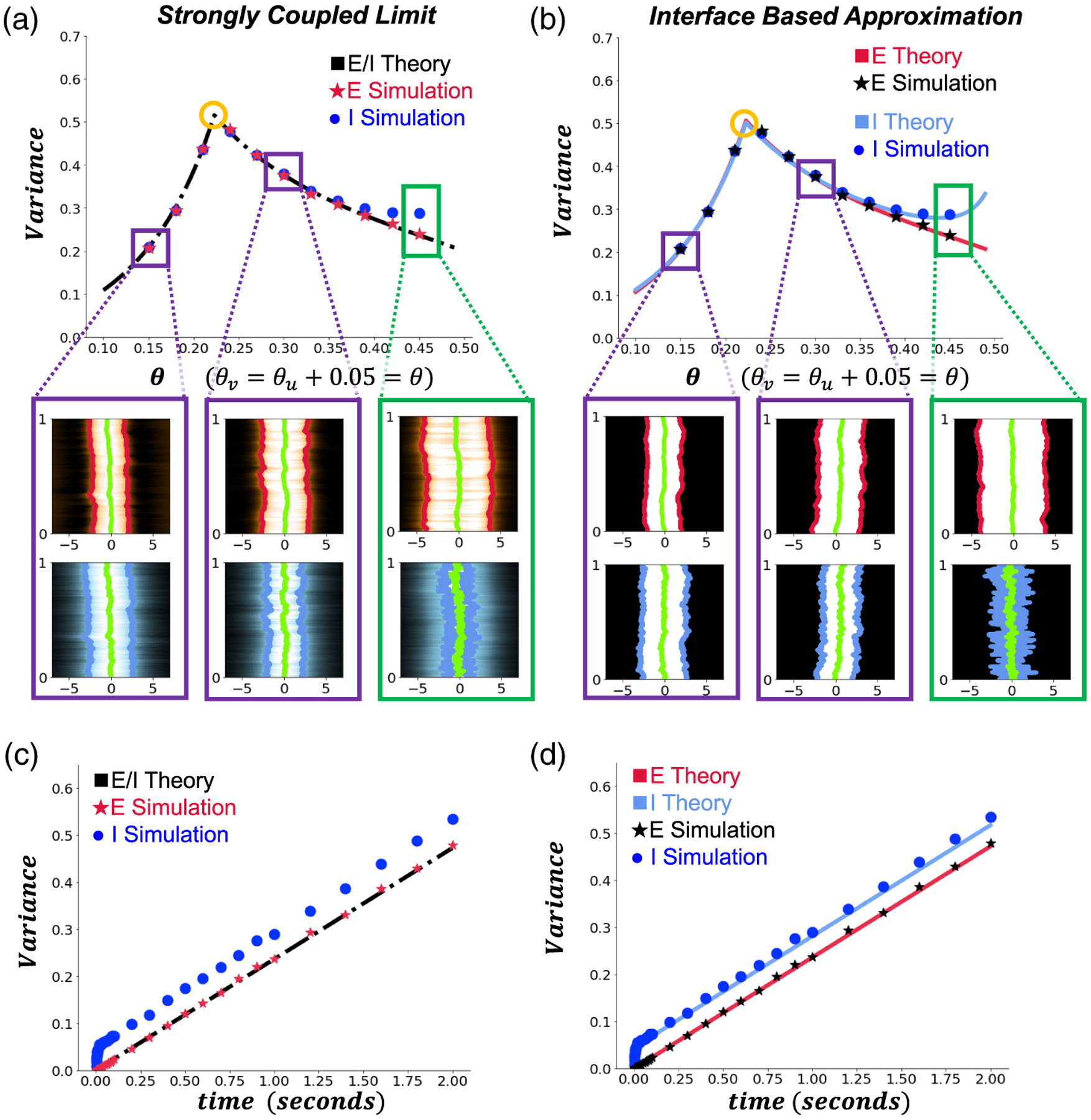
Variance predictions and simulations. Numerical simulations of (2.1) were run using an approximate version of the interface equations derived from (4.9). Euler-Maruyama was used for time-stepping with noise amplitude $ϵ=0.001$, the spatial interval was truncated to $[-3\pi ,3\pi ]$ with steps $dx=\frac{3\pi }{1000}$, timesteps are $dt=1ms$, and variances were calculated by marginalizing over 10⁴ realizations per point. (a) The strongly coupled limit prediction and corresponding simulations over 1 second. Although this prediction works reasonably well for small thresholds $\theta$, it breaks down for higher thresholds where the $I$ bump center of mass differs considerably, e.g., ${\theta }_u+0.05={\theta }_v=0.45$. Note the kink and change in the variance trend when $\theta$ passes through a value at which the half-widths $a_u$, a exchange order (gold circle). Insets show single $E$ (top panel) and $I$ (lower panel) bump simulations at indicated threshold values. $x$ is the horizontal axis and $t$ in seconds is the vertical axis. The E(I) bump interfaces at each step are shown by the red(blue) lines and the bump centers are represented by the green lines. (b) When comparing to estimates of variance made using the interface based approach, the theory more closely tracks the simulation results at higher firing rate threshold $\theta$. (c) The strongly coupled limit predicts pure diffusion and linearly scaling variance, which underestimates variance calculated from simulations at ${\theta }_u+0.05={\theta }_v=0.45$. (d) The interface based estimate tracks the drifting apart of the $E$ and $I$ bump, leading to more accurate variance predictions when ${\theta }_u+0.05={\theta }_v=0.45$. All other parameters are as in Table 1.