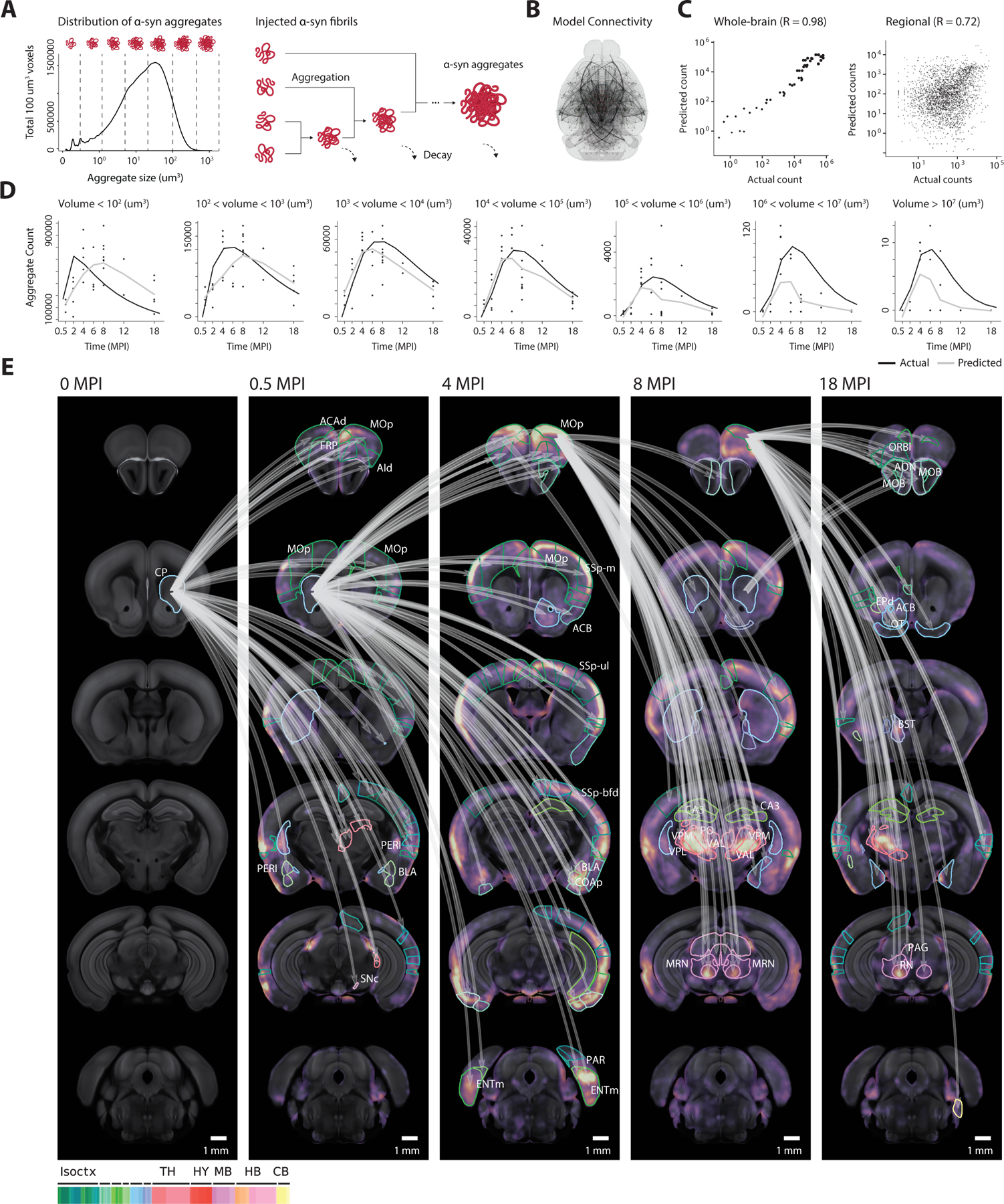
Figure 3. Computational model describes spreading, aggregation, and decay.

(A) To model the interactions between aggregates of various sizes, each aggregate’s volume is discretized into one of several size bins which are tracked as separate model variables in each region. Discrete-sized particles within each region can accumulate, with volumes combining additively. (B) The computational model describes the spreading of aggregates throughout the nodes of a directed graph, which relies on anatomical connectivity estimates from the Allen Connectivity Atlas. Each node represents an atlas region, with each edge representing the anatomical neuronal connectivity between the two regions. Thicker lines represent higher anatomical connections. (C) Fitted model accurately simulates both the longitudinal whole-brain counts of each discretized aggregate size (R = 0.98), and the regional counts (R = 0.72) for each size. (D) The raw time-series output from the computational model demonstrates the model’s ability to capture the dynamics of each discretized aggregate size. Black lines represent the model prediction of total aggregates of a given size, and gray lines represent the actual observed count. (E) Jacobian calculation between adjacent time points quantifies the model’s sensitivity to specific anatomical connections. The top 10% Jacobian elements for each pair of timepoints are displayed. Isoctx – isocortex, TH – thalamus, HY – hypothalamus, MB – midbrain, HB – hindbrain, CB – cerebellum. See also Figure S6.