



Abstract
This paper investigates how office-based physicians respond to Medicare reimbursement changes. Using variation from an Affordable Care Act policy that increased reimbursements for office-based care in four states, we use a triple difference analysis, comparing physicians with higher and lower reimbursement changes in treated states to similar physicians in untreated states. We find two mechanisms through which physicians respond. First, the reimbursement change affected integration—physicians with larger increases in office-based reimbursement were less likely to vertically integrate with hospitals and more likely to continue providing office-based care than physicians with smaller reimbursement increases. Second, we find some evidence that physicians who continued practicing in an office setting increased the volume of services provided.
Keywords: Medicare, Vertical Integration, Physician Reimbursement
1. Introduction
Medicare’s reimbursement schedule is an important policy lever to affect physician behavior. Physicians can potentially respond to changes in Medicare reimbursement through several mechanisms: by changing their volume of care, their practice intensity (e.g. the types of procedures they provide), or their relationships with other providers (e.g., vertical integration with hospitals). These various responses can have implications for costs, quality, and access to care.1 Understanding how volume and intensity margins interact with vertical integration behavior is increasingly important as United States physicians experience a wave of vertical integration—in 2021, 48.4% of physician practices were owned by hospitals, compared to only 13.6% in 2012 (Physicians Advocacy Institute, 2022, 2019). While a large literature has studied volume and intensity responses, only a small, recent literature has begun to study the impact of reimbursement on vertical integration. Further, we know of no research evaluating all three mechanisms in the same context.
We investigate how office-based physicians respond along these multiple dimensions to a Medicare reimbursement increase. We exploit a plausibly exogenous Affordable Care Act (ACA) policy that increased reimbursement rates for office-based care in four states (Montana, North and South Dakota, and Wyoming) in 2011. We estimate a triple difference (TD) analysis comparing physicians within affected states who were more and less exposed to the reimbursement increase and comparing similar physicians in unaffected states. Physicians responded to the rate changes along two margins. First, the reimbursement change affected integration—physicians with larger office-based reimbursement increases were less likely to vertically integrate and more likely to continue providing office-based care than physicians with smaller reimbursement increases. Second, physicians who continued practicing in an office setting increased the volume of services provided.
Our identification strategy leverages variation in reimbursement rates across time, physicians, and geographic areas. The ACA policy we leverage raised reimbursement rates on different office-based services unequally. Thus, even within a specialty, physicians in the four treated states were differentially exposed, depending on the bundle of services each physician performed. In these states, the reimbursement increases that physicians faced ranges from 3% to 15%. In addition to this variation across physicians, we also exploit variation across areas. For each county of our four treated states, we use covariate matching to identify similar counties in control states. We compare physicians in treated states to physicians from control states with the same specialty and who would have experienced similar reimbursement changes had they practiced in the treated states. The identification assumption for our triple-difference strategy is that physicians within specialty with similar practice styles prior to 2011 in treatment and control areas would have evolved similarly in terms of practice style and vertical integration, absent this ACA policy. Our results hold even if we just use variation in physicians in a traditional difference-in-difference, instead of using additional variation across geographies.
We find that the increase in office-based reimbursement caused an increase in the volume of care provided in an office-setting. This is driven by two mechanisms. First, the increase in office-based reimbursement caused a relative decrease in vertical integration. Office-based physicians can practice in either a traditional office setting or in a hospital-affiliated facility. Medicare reimburses procedures differently, depending on whether the procedure is administered in an office or in a facility. In our setting, physicians experiencing larger reimbursement increases specifically for services provided in the office setting were less likely to vertically integrate and more likely to continue providing office-based care. The second mechanism we observe is a change in the intensive margin of care—conditional on practicing in the office setting, physicians tend to increase their overall supply of care. We also look for changes in intensity of care (i.e., the types of procedures provided),2 but find no evidence for a systematic response on that margin.
We separately evaluate the responses of physicians operating in areas with varying population densities to explore the external validity of our results to other less rural states. We find that our results are largely robust across areas, suggesting that these results have some external validity. We also explore heterogeneity across physician specialties and ages. Supply responses appear largest among primary care physicians and surgical specialists. We further find that while physicians near retirement exhibit an increase in office-based care, vertical integration behavior is muted. This pattern is particularly striking for surgical specialists near retirement age who additionally exhibit an overall increase in Medicare participation, suggesting that for these physicians, increases in office-based reimbursement can delay retirement.
To explain why the reimbursement increase might both decrease vertical integration and for inframarginal physicians increase volume, we build a simple model of physician supply based on the model in Clemens and Gottlieb (2014). Physicians trade off profit against disutility of effort and choose between a independent office-based practice and vertical integration. This model combines our empirical estimates, suggesting that vertical integration accounts for a third of the total increase in office-based volume while the change in volume of inframarginal physicians accounts for the remainder. We use insights from our model along with Medicare reimbursement rate changes over time to understand how responses to reimbursement changes over time.
Related Literature:
This paper contributes to the literature evaluating how healthcare provision responds to changes in reimbursement.3 Most specifically, this paper relates to two strands of that literature on the impacts of Medicare reimbursement for outpatient care: first, the recent literature investigating how reimbursement impacts vertical integration and second, the broader literature estimating volume and intensity responses to Medicare reimbursement.
The relatively new literature on vertical integration and reimbursement tends to find that physicians vertically integrate when the reimbursement for care in facilities goes up relative to reimbursement for care in offices, though there are some counterexamples for specific procedures. The most closely related paper in this literature is Dranove and Ody (2019). This paper finds that increases in facility-based Medicare reimbursements relative to office-based reimbursement leads to vertical integration. Similarly, using longitudinal trends in site-specific payment rates, Post et al. (2021) finds that relatively higher Medicare reimbursement in facility settings is associated with vertical integration for primary care physicians and medical specialists. This literature suggests heterogeneity across providers and specialty: Post (2021), Sloan et al. (2021), Song et al. (2015), Masoudi et al. (2019), and Alpert et al. (2017) look at different segments of the market and some find responses while others do not.
In the large literature estimating volume responses to Medicare reimbursement for outpatient care, even the studies using clearly exogenous geographic level changes in reimbursement estimate both positive and negative volume elasticities. The seminal paper in this literature Clemens and Gottlieb (2014) exploits a 1997 nationwide change in the boundaries Medicare used to geographically adjust reimbursements. They find a positive response to reimbursement driven by volume and service intensity. However, Rice (1983) and Rice and McCall (1982) use similar older variation within Colorado in the 1980s and estimate a negative elasticity. Additional papers using non-exogenous reimbursement changes have found similarly mixed results (Brunt and Hendrickson, 2021b,a; Brunt, 2015; Hadley et al., 2009; Callaghan et al., 2016; Gruber et al., 1999; O’Neil et al., 2016; Shahinian et al., 2010; Jacobson et al., 2010; Yip, 1998).
This paper contributes to the literature in two ways. First, we provide novel evidence on the impact of office-based reimbursement changes on vertical integration behavior using plausibly exogenous increases in reimbursement. Our analysis suggests that the recent wave of vertical integration may be driven in part by the relatively low reimbursement rates in the office setting. Further, we find that increases in office-based reimbursement have a particularly large impact on the vertical integration decisions of primary care doctors and surgeons. These results are important for policy-makers considering the implementation of site-neutral payment that would equalize reimbursement across offices and facilities (Centers for Medicare and Medicaid Services, 2018; Cassidy, 2014).
Second, this paper is able to study vertical integration and volume of supply responses in the same context, tying together two previously separated literatures. Past studies have documented a variety of responses to reimbursement rate changes in different contexts.4 Studying both responses in the same setting provides a more complete characterization of the full impact of site-specific reimbursement changes, since one need not reconcile differences across settings and time-periods. As policy-makers consider changes to Medicare reimbursement policy, our analysis suggests that increases in office-based reimbursement would increase volume in that setting, but this would be partially offset by decreased facility volume driven by decreases in vertical integration.
The rest of our paper proceeds as follows. Section 2 describes background information on the Physician Fee Schedule and the ACA policy change. Section 3 describes the data. Section 4 outlines our triple-difference empirical strategy. Section 5 presents the results. Section 6 introduces a model and discusses the mechanisms. Finally, section 7 concludes.
2. Setting and Reimbursement Variation
We study office-based physicians in Montana, North and South Dakota, and Wyoming where an ACA provision increased reimbursement in 2011. We exploit this change in reimbursement, which had varying intensity across procedures and physicians, to understand how payment policies impact vertical integration as well as the volume of care.
2.1. Office-Based Physicians and their Medicare Reimbursement
We study office-based physicians because they have many mechanisms by which they can respond and they are likely particularly sensitive to Medicare reimbursement. Increases in office-based reimbursement could induce physicians to change not only their volume and intensity of care but also their vertical integration with hospitals. Office-based physicians typically own their own practice or are affiliated with a small provider group. These providers often have an option to vertically integrate their practice with a hospital and provide similar services in an outpatient facility. Increasing office-based reimbursement may make practicing in the office setting more lucrative, making physicians more likely to continue practicing in an office environment, thereby making them less likely to vertically integrate with other providers. Further, office-based physicians are likely highly responsive to marginal changes in Medicare reimbursement. In contrast to facility-based care, office-based care is more often provided by physicians with a financial stake in the office whose income is more closely linked to the Medicare reimbursement their procedures accrue. Office physicians likely have more room to self-refer and induce volume changes. Further, office-based care is paid at the procedure level—this granular payment scheme means that there is more scope for providers to vary provision than there is in other Medicare payment systems where multiple different procedures are bundled together into one payment.
Medicare sets reimbursement for office-based physicians in its Physician Fee Schedule (PFS). Reimbursement varies by both the procedure and the geographic region and is based on procedures’ input costs adjusting for geographic variation. All procedures are grouped into bins labeled with Current Procedural Terminology (CPT) codes—all procedures within a CPT are paid the same. Medicare determines the relative input costs for each CPT code separately for three types of inputs: provider work, practice expenses (materials, employee costs, and office rental), and malpractice liability insurance. The costs are quantified with relative value units (RVUs) so that each procedure has three RVUs whose sum describes the total cost of the procedure.
Input costs (RVUS) are separately adjusted for geographic variation in the costs of the inputs when setting reimbursement. Medicare divides the United States into localities,5 and for each of the three input types describes the costs within each locality with a geographic practice cost index (GPCI).
Medicare combines the input costs (RVUs) and geographic adjustments (GPCIs) to produce a CPT by locality specific reimbursement rate. A simplified version of the formula Medicare uses to combine the RVUs and GPCIs into procedure by locality reimbursement rates is below.6
| (1) |
In this equation, indexes procedure and indexes locality. The resulting product is scaled by a conversion factor that converts the RVUs to dollars.
2.2. Reimbursement Variation: ACA Floor on Geographic Adjustments
This analysis exploits an ACA policy that increased office-based Medicare reimbursement differentially across procedures. The ACA mandated a permanent floor for practice expense GPCIs in Frontier States: i.e., states where at least fifty percent of the counties have a population per square mile of less than six (Federal Register, 2010). There were five Frontier States in 2011: in one, Nevada, the floor did not bind, and in four, Montana, North and South Dakota, and Wyoming, the GPCI floor increased reimbursement from 2011 on—these are the four treated states.
Figure 1 shows that the increase in practice expense GPCI and reimbursement in the four treated states was large. Both RVUs and reimbursement rates are largely flat from 2007 to 2009, but in 2011, all treated frontier states have a GPCI of 1 and a correspondingly higher reimbursement rate. Note that reimbursement rates experienced a small increase in 2010, a year prior to the implementation of this policy. This 2010 increase is due to a separate, temporary ACA policy.7 As discussed in greater detail in section 4, our empirical strategies treat 2007 to 2009 as the pre-period and 2011 and later as our post period to avoid the issue of partial treatment in 2010.
Figure 1:

Variation in Practice Expense GPCI and Reimbursement Rates
Note: The left panel shows the practice expense GPCIs in the treated states where the 2011 GPCI floor was binding. In these states, the floor increased the GPCIs by about 10 to 15% relative to 2009. The right panel shows the actual reimbursement rates Medicare paid per RVU for office-based care—there was an approximately 15% increase.
In addition to increasing office-based reimbursements with the policy we exploit, the ACA also established floors for two parameters that increased inpatient and outpatient hospital reimbursement in Frontier states, but we argue that these policies will just slightly bias our estimated effects towards zero (111th Congress, 2010). The procedure level reimbursement increases in the office and outpatient facility setting have a small positive correlation.8 This means that while the absolute level of office reimbursement increased in 2011, the relative reimbursement in offices versus facilities increased slightly less in our setting than it would have had facility prices been held fixed. Physicians considering vertically integrating presumably respond to both absolute reimbursement levels in the office setting as well as relative reimbursement levels across office and facility settings. Because the presence of this facility price change mutes the response via the relative reimbursement channel, our vertical integration results will be biased towards zero. Given that the procedure level correlation with our price change is relatively weak, this bias is likely small. We discuss this in greater detail in appendix H.
Because the practice expense GPCI multiplies only the practice expense RVU in the reimbursement formula, the increase in reimbursement is larger for procedures with a larger share of RVUs from practice expenses. Comparing two procedures with very different practice expense shares exemplifies this distinction. Psychotherapy has a practice expense share of 0.23, while eye exams have a practice expense share of 0.75. For psychotherapy, a 15% increase in the practice expense GPCI would increase reimbursement by 4% since only a 0.23 share of the total RVUs are subject to the increased GPCI, while for eye exams the same 15% practice expense GPCI increase would increase reimbursement by almost 13% since a 0.75 share of the RVUs are subjected to the increased GPCI.9 Thus, the magnitude of reimbursement change faced by each provider will depend upon the bundle of procedures that they provide (see appendix G for more explanation).
3. Data and Variable Construction
This analysis uses both administrative Medicare claims data to measure utilization (volume, intensity, and place of service) as well as public Physician Fee-for-Service RVU files from the Centers for Medicare and Medicaid Services to measure reimbursement.
3.1. Physician Sample
The unit of analysis in our study is a physician. We construct our baseline sample of physicians using claims data from a random 20% sample of Medicare beneficiaries from 2007 to 2015. Because the reimbursement change of interest exclusively affected payments for office-based procedures, we restrict to physicians who primarily operated in an office setting in both 2008 and 2009. We classify a physician as primarily office based if 60% or more of their Fee-for-Service Medicare revenue is from an office-based setting.10
We categorize all specialties into primary care, medical specialties, surgical specialties, and other specialties based on the specialty codes in Machado et al. (2021), and within these categories, we define narrower groups to match the list of main specialties in Chan and Dickstein (2019). Appendix table A.3 lists how we bin specialty codes for our analysis. We drop all providers whose specialty does not match one of the main specialties or are not physicians.
For our main analysis, we exclude outlier physicians—physicians whose Medicare revenue in 2008 and 2009 was below the 5th percentile or above the 95th percentile among their specialty in treated states. We investigate the sensitivity of our results to these selection criteria in the appendix. Table 1 shows the number of office-based physicians and their Medicare revenue separately by specialty for the most common specialties in our sample.
Table 1:
Physicians in Treated States
| Reimbursement Change (%) | ||||||
|---|---|---|---|---|---|---|
| Number | Total Revenue | Mean PE Share | Mean | 10%-ile | 90%-ile | |
| Total MDs | 2658 | 55.83 | 0.55 | 0.094 | 0.07 | 0.127 |
| Primary Care | 995 | 18.72 | 0.49 | 0.082 | 0.069 | 0.095 |
| Family medicine | 712 | 11.60 | 0.49 | 0.081 | 0.070 | 0.092 |
| Internal medicine | 260 | 6.99 | 0.48 | 0.082 | 0.068 | 0.097 |
| Medical Specialists | 414 | 15.80 | 0.60 | 0.104 | 0.079 | 0.132 |
| Dermatology | 41 | 2.95 | 0.59 | 0.099 | 0.0846 | 0.114 |
| Cardiology | 116 | 4.57 | 0.60 | 0.106 | 0.079 | 0.132 |
| Oncology | 55 | 3.07 | 0.65 | 0.115 | 0.088 | 0.135 |
| Neurology | 62 | 1.65 | 0.58 | 0.101 | 0.081 | 0.133 |
| Surgical | 915 | 14.11 | 0.56 | 0.097 | 0.079 | 0.115 |
| Ophthalmology | 80 | 3.24 | 0.52 | 0.086 | 0.077 | 0.093 |
| Orthopedic surgery | 251 | 4.30 | 0.57 | 0.1 | 0.081 | 0.120 |
| Urology | 65 | 2.71 | 0.59 | 0.1 | 0.088 | 0.109 |
| General surgery | 180 | 1.40 | 0.60 | 0.104 | 0.076 | 0.145 |
| Otolaryngology | 72 | 1.03 | 0.58 | 0.099 | 0.083 | 0.114 |
| Obstetrics and gynecology | 168 | 0.68 | 0.54 | 0.091 | 0.073 | 0.104 |
| Neurosurgery | 41 | 0.24 | 0.53 | 0.088 | 0.066 | 0.123 |
| Other | 334 | 7.19 | 0.56 | 0.099 | 0.045 | 0.154 |
| Radiology | 92 | 3.37 | 0.70 | 0.125 | 0.062 | 0.155 |
| Pathology | 47 | 1.12 | 0.47 | 0.084 | 0.035 | 0.145 |
| Psychiatry | 103 | 0.97 | 0.35 | 0.057 | 0.042 | 0.076 |
Note: This table lists the common specialties nested into larger categories for our main sample after imposing the restrictions described in section 3.1. The first column shows the number of distinct providers with office-based care in both 2008 and 2009. The second column lists revenue in millions of dollars—it is the sum of all office-based Medicare reimbursements for our 20% sample of patients in 2008 and 2009. The third column shows the average practice expense share of services provided by each specialty. Finally, the last column shows the distribution of the projected reimbursement change within each specialty. The reimbursement changes include only the changes induced by the exogenous GPCI floor—we calculate these by applying 2009 and 2011 GPCIs to 2009 RVUs and procedure bundles. All physicians are weighted equally.
Figure 2 shows that during this time, there was broad movement of Frontier state physicians out of office-based care and into facility based care. Per our inclusion condition, all physicians in the sample provided office-based claims in 2008 and 2009. However, in the subsequent years, a portion of physicians move out of office-based practice and a small subset do not have any attributed claims at all.11 Further, during this period some of our sample’s physicians moved towards facility-based care as the share of physician providing only facility-based claims increases over time.12
Figure 2:
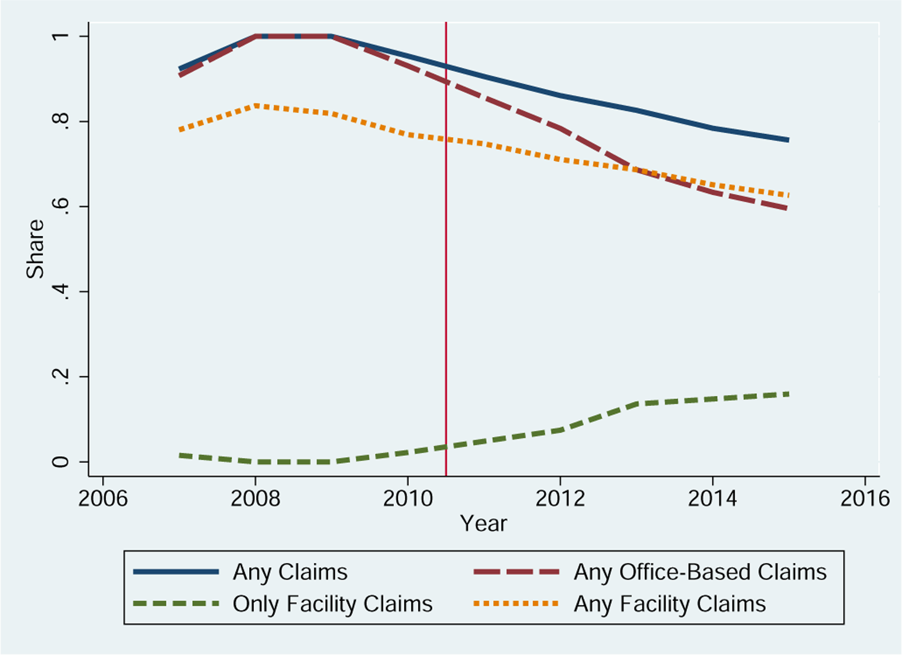
Physician Participation in Medicare Over Time
Note: This figure has participation rates in various types of care for the baseline sample of physicians. The share with any claims and with office-based claims is mechanically 1 in 2008 and 2009 because that is part of the inclusion criteria. This figure shows that participation falls off with time, especially for office-based care. This appears somewhat driven by an increase in facility-only claims. Physicians are weighted equally.
3.2. Physician Level Reimbursement Change
We construct a physician-specific measure of reimbursement change generated by the statutory change. This measure of reimbursement change depends only on the composition of procedures physicians performed before the policy (and not their endogenous responses to the policy).
We use the CMS Physician Fee-for-Service RVU files, which contain RVUs, GCPIs, and the annual conversion factor that define the statutory reimbursements for each procedure in each locality each year. We select the most revised January publication each year and use the reimbursement formula in the annual documentation accounting for any special adjustments that apply to calculate rates.13
We calculate physician level reimbursement changes that include only reimbursement variation caused by the Frontier State practice expense GPCI floor. Both the plausibly exogenous policy and endogenous changes in RVUs, other adjustments, and procedure bundles affect physician reimbursement over time. We isolate the exogenous variation by holding RVUs and procedure bundles fixed at the pre-period levels and only varying the GPCIs.
To isolate the exogenous variation in reimbursement, we first calculate the impact of the GPCI floor on each procedure’s reimbursement: we hold fixed the RVUs at their 2009 level and calculate the percent change between the total reimbursement with the 2009 and 2011 GPCIs. Next, to aggregate the reimbursement changes to the physician level, we weight the procedure level changes by the procedures in the bundle that each physician provided in the pre-period office-based claims. For the pre-period claims, we use all office-based claims from 2008 and 2009. The two year window reduces noise (some physicians have low volumes, and we only have a 20% sample of claims). We do not use 2010 because there was a small increase in GPCIs that may have impacted quantities. We excluded the few facility-based claims that these physician perform in calculating the reimbursement rate change since that is less relevant to their decisions about office-based provision. This process is explained in more detail in the appendix A.1.
For physicians in the matched control counties, we define the counterfactual reimbursement rate changes they would have faced if they had practiced in the treated states. As seen in appendix J, the distribution of counterfactual reimbursement rate changes is quite similar to the distribution of changes the treated physicians faced suggesting that the groups are comparable.
Table 1 shows that there is variation in physician level reimbursement rate changes both within and across specialty. Within most specialties there are a few percentage points of variation in the rate changes. For example, for family medicine physicians (the most common specialty) the 10th percentile reimbursement increase was 7% and the 90th percentile was 9.2%. Histograms show the complete distributions of the change in reimbursement for some of the most common specialties in appendix figure A.1.
3.3. Measuring Physician Responses
We study two types of responses to an increase in reimbursement for office-based visits: changes to office-based care and changes to vertical integration and overall supply.14
For office-based care, we measure participation, volume, and service intensity. We characterize a physician as participating in office-based care if they have any claims with an office place of service code. We measure volume by total RVUs provided to incorporate both changes to service counts and to the intensity of the procedures. RVUs are designed by Medicare to measure the relative input costs across procedures, and summing RVUs across procedures is a standard way to measure total volume (Clemens and Gottlieb, 2014).15 Similarly, we measure the intensity of office-based procedures by RVUs per procedure.
We measure vertical integration by provision of facility-based care. Since many office-based physicians provide some facility based-care (for example visiting their patients in the hospital), we follow Neprash et al. (2015) and measure vertically integrated physicians as those who switch to only facility-based care (and provide no office-based care).
Finally, we measure aggregate provision both by looking for any participation in Medicare and total volume. We consider a physician to be participating in Medicare if they have any claims in our dataset regardless of place of service. Total volume is measured using the count of total services performed across facility and office settings. We use this measure, rather than RVUs, because RVUs are reported for a subset of input costs for facility-based claims.16
Unadjusted timeseries of these outcome measures for Frontier and non-Frontier state physicians can be found in appendix figures A.3 and A.4.
4. Empirical Strategy
Our main specification is a triple-difference that exploits variation in timing, area, and the practice expense share (PE share). The policy change caused larger reimbursement rate increases for high PE share physicians in treated states, while control areas and low PE share physicians had lower reimbursement increases. Our identifying assumption is that the difference in outcomes within specialty between high and low PE share physicians would have been parallel across treated and control areas over time.
4.1. Comparing Similar Physicians
To increase the plausibility of our identifying assumption, we compare physicians only within (rather than across specialty), and we select control areas with covariate matching so that they are similar to the treated states.
4.1.1. Within Specialty Variation
Our specification compares physicians within specialty groups who receive smaller and larger reimbursement changes. We assume that physicians are on parallel trends only within specialty, not across specialties. The variation in physician reimbursement changes is driven by pre-policy variation in procedure bundles across physicians—due to some combination of patient needs and practice style. Physicians with higher reimbursement increases are those with more high practice expense share procedures, thus specialties have different average reimbursement changes. For example, psychiatrists tend to provide less practice expense intensive care and hence have lower reimbursement increases than cardiologists who do more imaging and testing. Given potential differences across specialties, we exclusively use within-specialty variation.
4.1.2. Covariate Matching to Select Control Group
We use covariate matching to select counties that are similar to the counties in the treated states. To select control counties, we start with the pool of all counties in Nevada (a Frontier State where the policy did not bind) and the states surrounding the treated states. We follow a covariate matching procedure closely paralleling Diamond et al. (2020). We generate a propensity score for each county by regressing a treatment indicator on many covariates17, and select the five most predictive: 2010 poverty rate, SNAP recipiency rate, share of population living on farms, number of hospital beds per capita, and psychiatrists per capita. We match each treatment county to the five control counties with the closest propensity score and weight them proportionately to their FFS population and the FFS population of their matched treatment county (we allow control counties to match multiple treatment counties).
We include all physicians practicing in the matched control counties. We define counterfactual reimbursement rates changes that they would have faced had they practiced in an average treated state based on their PE share. The distribution of the counterfactual reimbursement rate changes is quite similar to the distribution the treated physicians faced, suggesting the groups are comparable.
More details about this method as well as summary statistics are in appendix J.
4.2. Triple Difference Estimating Equation
Our baseline triple difference specification is the following:
| (2) |
Where indexes physicians; , specialty; , area (treated or control); and , year. is the physician level reimbursement change, are physician fixed effects, and are separate specialty by year fixed effects for treated and control areas. The individual physician fixed effects implicitly include specialty since that is a physician level attribute. Standard errors are clustered at the physician level—this accounts for any serial correlation in physician outcomes that is not absorbed by the physician fixed effects. For our baseline specification, we weight the treatment physicians equally (and control physicians by the weight of their county described in the covariate matching section above)—though we consider robustness to weighting by Medicare spending. See appendix figure A.2 for the “first stage” of reimbursement per RVU in this triple-difference specification.
The coefficients identify the causal effect of a change in reimbursement rate on outcome under the assumption of parallel differences in outcomes across treatment and control areas. This is the change relative to the omitted time period. In our event studies plots, we omit year 2009.That is, we assume that in both treatment and control states, the relative outcomes of physicians with high compared to low would have evolved similarly absent the policy change. This assumption allows us to net out changes in relative outcomes between high and low physicians due to mean reversion and other factors present in both treatment and control states. Under this assumption, changes in the relative outcomes of high and low in treated states that are in excess of changes in control states can be attributed to the reimbursement change.
This assumption is impossible to validate, but confirming an absence of pre-trends provides some evidence. See appendix section B for unadjusted timeseries of outcomes.
We present the results from the above regression in event study plots in the next section. We also run a version where we group years together into a pre-period (2007 to 2009), a short run post-period (2011 to 2012), and a long run post-period (2013 to 2015) to increase power and summarize the results. In this binned regression we omit the pre-period, so coefficient are relative to the average in the per-period. Additionally, we omit 2010 since that year had a partial treatment that physicians knew was temporary.
4.2.1. Alternative Specification: Difference-in-Difference
In addition to our main triple-difference (TD) specification, we also present difference-in-difference (DID) results (appendix section C). This specification compares physicians in treated states within specialty groups who receive smaller and larger reimbursement changes. We can use the DID approach to examine the trends of providers with different levels of exposure to the reimbursement change in our treatment and control group separately. This allows us to see how large the deviation from parallel trends is within the treatment group that is solved by our TD. In the context of the DID, the control group is thus used as a falsification to validate the DID parallel trends assumption. For more details on the DID specification, see appendix D.
5. Results
Our results show that increased reimbursement in the office setting leads to increases in office-based provision. This is driven by a decrease in vertical integration (i.e., movement to facility-only provision). There is some evidence of an increase in care volume and no evidence of a systematic change in service intensity.
5.1. Impacts on Participation and Vertical Integration
Figure 3 and the first three columns in table 2 show that increases in reimbursement rates for office-based care increased the provision of office-based care, decreased vertical integration, and had minimal impact on total participation.18
Figure 3:

Practice Location and Overall Medicare Participation
Note: This figure has the results from equation 2, the TD model comparing physicians based on the percent increase in reimbursement rate and treatment status of the state of the physician’s practice. The outcomes are indicated in the captions. Physicians are weighted equally. Standard errors are clustered at the physician level. The error bars show 95% confidence intervals. The mean of the outcome variable for the treated physicians in 2009 are below each figure. The dashed vertical line indicates the end of the pre-period, and the solid vertical line indicates the beginning of the post-period. All estimates are relative to 2009.
Table 2:
DDD Results
| (1) (Office) |
(2) 1(Facility) |
(3) (Any) |
(4) Ln(Office RVUs) |
(5) Ln(Office RVUs/Service) |
(6) Ln(Total Services) |
|
|---|---|---|---|---|---|---|
| 1–2 year | 0.618 (0.462) |
0.0264 (0.247) |
0.628 (0.409) |
−0.851 (1.846) |
1.008 (0.562) |
−1.248 (1.085) |
| 3–5 year | 1.955 (0.539) |
−1.549 (0.340) |
0.394 (0.480) |
4.986 (2.071) |
−0.970 (0.882) |
0.442 (1.204) |
| 2009 Mean (Treated Obs) | 1 | 0 | 1 | 5.63 | 0.68 | 5.29 |
| N Providers Treat | 2658 | 2658 | 2658 | 1306 | 1306 | 1784 |
| N Providers Control | 14053 | 14053 | 14053 | 9069 | 9069 | 10160 |
Note: This table has the results from equation 2 with the year indicators grouped in a pre-period, a 1–2 years post, and a 3–5 years post period. Columns 1 though 3 have the results for practice locaiton and overall practice location (analogous to figure 4)—an indicator for any office-based claims, an indicator for practicing only in a facility, and an indicator for having any Medicare claims at all. Column 4 and 5 have the log RVUs in offices to measure office volume and the log of RVUs per service to measure office intensity. Column 6 has the results on total care—the log of service counts in either the office or facility setting. Below the regression results, we present the 2009 mean of the outcome variable in the treated states and the number of unique providers in the regression. Each estimate is relative to the pre-period (2007 to 2009).
Figure 3, panel (a) and the first column of table 2 shows that physicians with higher reimbursement increases were more likely to continue providing office-based care in the long run. We measure office-based provision using an indicator for any office-based claims. The coefficient can be interpreted as the percentage point change in physician participation caused by a 1% reimbursement increase. We see that a 1% reimbursement increase causes a 1.96 percentage point increase three to five years after the reimbursement change.
We measure vertical integration by an indicator for providing only facility-based care, so the coefficient is again a semi-elasticity—a 1% increase in office-based reimbursement decreases vertical integration by about 1.55 percentage points. Comparing the magnitude the effect on office-based participation, we see that the decrease in facility-based participation is almost as large in magnitude as the increase in office-based care. This suggests that our extensive margin response of office-based provision is largely driven by a decrease in vertical integration.
Our analysis suggests that the increase in office-based participation is almost completely driven by decreases in vertical integration, as the impacts on these two types of provision are almost equal in magnitude with opposite sign. When we look at the outcome of any Medicare participation across places of service in panel (c) of figure 3, the results are a noisy null. Though the upper bound of the confidence intervals includes a semi-elasticity above 1, which is substantial.
5.2. Impacts on Intensive Margin and Aggregate Care
We next investigate intensive margin responses to reimbursement and find suggestive evidence that higher reimbursement increases the volume of office-care provided for inframarginal physicians (though these results have some pre-trends). We find no evidence of changes to service intensity.
To evaluate how physicians who remain in office-based care respond to reimbursement changes we use log RVUs as our outcome and limit our sample to the balanced panel of physicians always participating in office-based provision. Since our outcome is logged, the coefficient can be interpreted as an elasticity—it is the change in a logged outcome from a percent in change in the exogenous variable. The results are shown in figure 4, panel (a). There are significant pre-trends which are concerning, but it is suggestive that there may be some long run increase in volume. The pre-trends are likely due to the extensive margin change in office participation—the composition of the physicians who remain in office based practice is likely different in treatment and control areas since vertical integration decreased in treatment areas.19 We present the balanced panel despite this bias because the results for the unbalanced panel include both intensive margin responses as well as selection into participation, and our results suggest that selection into participation is large, so it is hard to interpret those results. However, we present the unbalanced panel in appendix figure A.7, and there are no pre-trends, which suggests that the problem is indeed driven by by the compositional difference between the treatment and control areas in the balanced panel. We additionally present alternative measures of intensive margin results estimated on both a balanced panel and an unbalanced panel (figure A.7 and A.8).
Figure 4:

Care Volume and Service Intensity
Note: This figure has the results from equation 2, the TD model comparing physicians based on the percent increase in reimbursement rate and treatment status of the state of the physician’s practice. The outcomes are indicated in the captions. Physicians are weighted equally. Standard errors are clustered at the physician level. The error bars show 95% confidence intervals. All regressions are on the balanced panel of physicians always participating in the relevant care type. The mean of the outcome variable for the treated physicians in 2009 are below each figure. The dashed vertical line indicates the end of the pre-period, and the solid vertical line indicates the beginning of the post-period. All estimates are relative to 2009.
To investigate the impact on intensity of office-based care, we use the outcome log RVUs per service. We again restrict to a balanced panel so that the effect is not confounded by selection into office-based care (thus, this regression is subject to the same biases we discuss for the office-based volume). However, there is no evidence of the problem showing up in pre-trends. In contrast to the findings of Brunt (2015) and Clemens and Gottlieb (2014), we find no evidence of a response. We discuss potential reasons for this result in section 6.
Finally, we measure total volume (across office and facility settings) by the total number of procedures that physicians provide (panel (c)). We estimate this on a balanced panel of physicians who participated in Medicare for the entirety of the sample. The event study has a significant pre-trend, but there is no evidence of a systematic increase in total care. In the appendix, we present a number of alternative estimates of the effect of this reimbursement change on total provision across facility and office settings. Figure A.9 shows the impact of the reimbursement change on the log of total patient visits and the log of total unique patients on the balanced panel. Figure A.10 shows the effect of all three measures on an un-balanced panel. Finally, figure A.11 shows the effect for the levels of all three variables, including zeros. Across all versions, we see little evidence of a systematic increase in overall provision.
5.3. Robustness
Our most important robustness check is to consider the alternative DID specification. Here we do not need to assume parallel trends across treatment and control areas and can instead use the control area event study as a falsification test for the parallel trends assumption within specialty. For this method we only need to assume parallel trends within physician specialty in treated states. The DID results (in appendix C) are fairly similar to the TD results in the treatment group (though the pre-trends are slightly worse) and very small and insignificant in the control group. Reassuringly, this suggests that the treatment group drives the results while the control group simply accounts for slight differences in trends.
We explore several variations in sample selection, and the results are relatively robust. For the intensive margin outcomes, we consider a number of alternative measures—we measure volume by the number of services, patient visits, or annual distinct patients rather than by RVUs—estimated separately on an unbalanced and balanced panel of physicians who are always active (appendix figures A.7 and A.8, respectively). Similarly, for our analysis of total care provision (across office and facility settings), we present several measures on both balanced and unbalanced panels of physicians (see figures A.9, A.10, and A.11). Qualitatively, our results are similar in that we find evidence of an increase in the volume of office-based care but no evidence of a systematic increase in total care across all settings.
We also conduct robustness to test the sensitivity of our results to our baseline sample restrictions. We drop only low volume outliers and include all physicians with high Medicare revenue (appendix figure A.12). We drop the bottom 25% of small volume physicians—these have noisier estimates of the reimbursement rate change (appendix figure A.13). We include all physicians, even those who are not majority office-based (appendix figure A.14). We restrict to physicians, who receive at least 80% of their Medicare revenue in office-based settings (appendix figure A.15). We weight the analysis by each physicians’ Medicare revenue (appendix figure A.16). None of these variations make a big difference in the results.
5.4. Heterogeneity
We examine heterogeneity along three margins: specialty, age, and population density. Older physicians have similar increase in office-based care, but smaller decreases in vertical integration, suggesting that retirement timing is affected. Further, the results do not vary much with population density bolstering confidence in their external validity.
Heterogeneity by Specialty:
We next examine responses for broad specialty categories, grouping physicians into primary care, medical specialists, and surgical specialists following Machado et al. (2021). The results are shown in the top three panels of table 3 with the event study plots in the appendix figures A.18 to figure A.20.
Table 3:
Heterogeneity
| (1) (Office) |
(2) (Facility) |
(3) (Any) |
(4) Ln(Office RVUs) |
(5) Ln(Office RVUs/Service) |
(6) Ln(Total Services) |
|
|---|---|---|---|---|---|---|
| Primary Care | ||||||
| 1–2 year | −0.198 (0.914) |
0.0553 (0.628) |
−0.154 (0.755) |
3.248 (4.316) |
0.389 (1.175) |
5.122 (2.100) |
| 3–5 year | 2.385 (1.028) |
−2.699 (0.758) |
−0.433 (0.820) |
9.001 (4.048) |
0.843 (1.376) |
8.785 (2.108) |
| 2009 Mean (Treated Obs) | 1 | 0 | 1 | 5.48 | .54 | 5.23 |
| N Providers Treat | 995 | 995 | 995 | 427 | 427 | 665 |
| N Providers Control | 5622 | 5622 | 5622 | 3415 | 3415 | 3996 |
| Medical Specialists | ||||||
| 1–2 year | 0.683 (0.975) |
0.405 (0.479) |
1.087 (0.883) |
−2.353 (3.273) |
1.064 (0.890) |
−6.146 (2.088) |
| 3–5 year | 0.678 (1.137) |
0.0641 (0.712) |
0.742 (1.011) |
7.491 (4.773) |
−0.431 (1.182) |
−4.793 (2.486) |
| 2009 Mean (Treated Obs) | 1 | 0 | 1 | 6.49 | .73 | 6.10 |
| N Providers Treat | 414 | 414 | 414 | 234 | 234 | 304 |
| N Providers Control | 2680 | 2680 | 2680 | 1961 | 1961 | 2088 |
| Surgical Specialists | ||||||
| 1–2 year | 0.807 (0.890) |
−0.0875 (0.387) |
0.723 (0.816) |
1.130 (2.603) |
0.220 (1.084) |
−0.397 (1.569) |
| 3–5 year | 3.513 (1.096) |
−2.574 (0.706) |
0.941 (1.017) |
2.769 (3.940) |
−0.663 (1.312) |
3.228 (2.119) |
| 2009 Mean (Treated Obs) | 1 | 0 | 1 | 5.34 | .73 | 4.87 |
| N Providers Treat | 915 | 915 | 915 | 500 | 500 | 616 |
| N Providers Control | 3884 | 3884 | 3884 | 2623 | 2623 | 2843 |
| 60+ MDs | ||||||
| 1–2 year | 0.250 (0.989) |
−0.0446 (0.509) |
0.215 (0.902) |
1.488 (3.948) |
0.895 (1.099) |
2.149 (2.761) |
| 3–5 year | 1.885 (1.134) |
−0.882 (0.523) |
1.005 (1.053) |
7.352 (4.923) |
−0.419 (1.854) |
2.642 (2.980) |
| 2009 Mean (Treated Obs) | 1 | 0 | 1 | 5.75 | .59 | 5.43 |
| N Providers Treat | 689 | 689 | 689 | 271 | 271 | 359 |
| N Providers Control | 3467 | 3467 | 3467 | 1730 | 1730 | 1917 |
Note: Similar to table 2, this table has the results from equation 2 with the year indicators grouped in a pre-period, a 1–2 years post, and a 3–5 years post period. Columns 1–3 show numeric results corresponding to figures 3 and 4 has an indicator for any office-based claims. Column 2 the log RVUs in offices to measure office volume, and the log of RVUs per service to measure office intensity. Column 4 has the results for an indicator for facility only claims, which can be interpreted as vertical integration. And columns 5 and 6 have the results on total care—an indicator for any claims at all and the log of service counts. Below the regression results, we present the 2009 mean of the outcome variable in the treated states and the number of unique providers in the regression. Each panel presents separate regression results for different sub-samples of physicians. The top three panels separate physicians by their specialty group. The bottom panel includes all physicians who were at least 60 years old in 2011. Each estimate is relative to the pre-period (2007 to 2009).
Primary care physicians respond to reimbursement changes similarly to physicians in general with the exception that total volume across places-of-service increases on the intensive margin. For medical specialists the results are rather noisy, but there are relatively few medical specialists in the treated states.
For surgical specialists, the increased reimbursements caused increased extensive margin participation to a larger extent than for physicians on average. Surgeons respond less on vertical integration margins, so increases in office-based provision are more driven by an aggregate increase in participation. We similarly observe intensive margin reimbursement increases do not seem to cause an increase in provision.
Heterogeneity by Age:
Older physicians have retirement as an option in addition to their choice of practice style and volume. Among physicians who were at least 60 years old in 2011 when the reimbursement increased, there is a similar extensive and intensive margin increase in office-based provision as there is in the general population, though the former effect is not statistically significant. Looking at the effect on vertical integration, we find a statistically insignificant decline in facility-based provision. Further, the point estimate is smaller in magnitude than the general population. These results suggest that for these older physicians, the reimbursement increase drove an increase in office-based provision largely through the intensive margin of volume rather than a decrease in vertical integration.
In appendix figure A.20, we find further evidence of heterogeneity. While surgeons younger than 60 exhibit large decreases in vertical integration, surgeons approaching retirement exhibit no response. Further, older surgeons also appear to exhibit an extensive margin response, increasing their overall participation in Medicare. While noisy, these results suggest that increasing payment rates can also impact supply by delaying retirement for certain physicians.
Heterogeneity by Population Density:
The rural nature of our treatment states could limit the external validity of our results. To address this, we repeat our analysis restricting to the higher population density areas of the treated states. We find that the impact is relatively stable in the sub-samples with higher population density.
To evaluate how the results change with population density, we repeat the analysis, progressively restricting to higher density areas, and compare the results. We summarize the impact on participation, volume, and vertical integration by running a pre/post triple-difference. These results are shown in figure 5—for all three outcomes of office-based participation, office-based volume, and vertical integration the results are relatively stable with population density though the standard errors increase as the sample size decreases.
Figure 5:

Long-Run Triple-Difference Coefficient by Population Density
Note: This figure has the results from equation 2, the TD model comparing physicians based on the percent increase in reimbursement rates in treatment versus control counties. It presents the long-run (i.e. 3 to 5 year) post-policy coefficient, analogous to the result from table 2. The outcomes are indicated in the captions. Physicians are weighted equally. Each point on the graph is from a separate regression that successively reduces the number of physicians restricting to those from higher population density counties—the leftmost point includes the full sample, the next the top 75%, the top 50%, the top 25%, and the top 10%. The error bars show 95% confidence intervals. Each point has the number of physicians and the population density (in people per square mile) for the cutoff in the x-axis.
6. Model: Interpreting the Empirical Findings
To evaluate the relative magnitudes of the two mechanisms affecting office-based volumes (vertical integration and changed volumes among inframarginal office-based physicians), we develop a simple model for how physicians respond to financial incentives. This model yields an intuitive way to combine our elasticity estimates from the previous sections, which suggests that the change in volume of inframarginal physicians accounts for two-thirds of the effect on office-based care while the change in vertical integration accounts for the remainder. Finally, we discuss how this model could explain why the mechanisms for physician responses to reimbursement rate changes are different in our paper and Clemens and Gottlieb (2014) (CG). This framework focuses on office-based care and does not consider facility-based or total care.
6.1. Modeling Office-Based Provision
Our model is a variation of CG’s model. Like CG’s, it describes altruistic physicians choosing their practice style as well as volume of care. However, we model physicians as choosing between either a non-integrated office-based practice style or a vertically integrated style where physicians are employed by facilities and provide only facility-based care (CG model physicians choosing between standard and intensive practice styles). We focus on the integration choice because our empirical analysis shows integration as a significant alternative to office-based practice and the literature suggests that it is becoming increasingly common (Baker et al., 2018; Capps et al., 2018; Neprash et al., 2015).
Model Setup20
Physicians value revenue net of costs, patient health benefits (altruism), and have disutility from effort. Each physician has some productivity (distributed according to distribution )—physicians can produce one unit of care with effort .
Physicians choose between a non-integrated office-based practice style and a vertically integrated style . Physicians choosing the non-integrated style provide office-based care and receive reimbursement per unit of care with a variable cost per unit, —they choose a quantity , and thus, have total profits . Producing units of care incurs disutility cost where is increasing and convex. Physicians value the patient health benefit— denotes utility from marginal health benefit of care (positive but decreasing), where , the total care produced by all physicians, is taken as given by individual physicians.
Physicians choosing the vertically integrated style receive a fixed wage from the facility that employs them and pay no marginal costs—they also provide no office-based care as all their care is facility-based. We assume that their employer requires them to exert a fixed amount of effort producing facility-based care, and that they have a fixed altruistic benefit from their employment. Thus, vertically integrating is a constant outside option, denoted .
We assume that physicians are the sole decision makers and that patient demand can be ignored. This is consistent with either excess demand or provider induced demand. Because the overall response to reimbursement rates is positive, this seems like a reasonable assumption.
Assuming utility is quasilinear, the utility from each practice style is
In equilibrium, each physician chooses either style or , and those choosing also choose some optimal quantity of care . These choices are a function of individual physician productivity () and the reimbursement rate and cost ( and ). We solve the model in detail and prove the following results in appendix M.
Model Results
This model yields three key results. First, there is a threshold productivity () such that physicians with productivity above the threshold () choose practice style while those below choose . Second, this threshold is decreasing in reimbursement () so that when reimbursement is higher, fewer physicians integrate . Third, conditional on choosing practice style , physicians provide more office-based care when is higher .
The relationship between office-based volume and reimbursement incorporating both the integration and the change in volume for inframarginal office-based physicians is governed by the following derivative, in which both terms are positive.
| (3) |
Figure 6 shows an example of what quantities of healthcare supplied might look like under this model and how they would change as reimbursement or profit margins for independent practice change. The blue curve shows a possible initial state. Low productivity physicians are vertically integrated and provide no office-based care. There is a threshold productivity () above which physician choose the non-integrated practice style and provide office-based care. The red curve shows the impact of a reimbursement increase. Increasing the reimbursement causes non-integrated physicians to provide more care and causes some integrated physicians to become non-integrated and increase their office-based volume. Inframarginal vertically integrated physicians are unaffected by the reimbursement change as they provide only facility-based care and are paid a fixed wage.
Figure 6:

Practice Style, Volume, and Reimbursement
Note: This figure shows an example of how physicians in the model change their provision and practice style as the reimbursement changes. Note that higher productivity physicians provide more care than low productivity ones—the discrete jump is when physicians switch from integrated to independent. Within office-based care, provision increases due to altruism and profit motives. Increasing reimbursement causes independent style physicians to provide more care and causes some integrated physicians to become independent and increase their volume discretely. Inframarginal integrated physicians are unaffected by the reimbursement change.
6.2. Applying the Empirical Estimates to the Model
The empirical section of this paper found the volume elasticity for office-based physicians and the semi-elasticity of office-based participation. These quantities can be combined using the decomposition in equation 3, with some rescaling.
We scale the derivative in equation 3 to an elasticity and reformulate it in terms of the empirical quantities we estimated (see appendix M for details). Assuming that the elasticity of volume with respect to reimbursement and volume itself are constant across office-based physicians, the aggregate elasticity is the following.
| (4) |
The total quantity is approximately the individual quantity per physician times the number of physicians. Thus, the total change is approximately the sum of the percent changes in each. And multiplying the change in participation by the inverse of the share still participating converts it from a percentage point to a percent change.
Plugging the empirical results into equation 4, yields a long run elasticity of total office-based quantity with respect to reimbursement of approximately 7.43. This is the sum of the 4.986 elasticity among inframarginal office based physicians (see the long run estimates in table 2) and , where 1.955 is the semi-elasticity of office-based participation (table 2) and 0.8 is the approximate share participating in office-based care after 3 years (figure 2). Thus, our point estimates suggest that the integration mechanism accounts for roughly a third of the response. However, our estimate of the elasticity of office-based care among inframarginal office based physicians is quite noisy. A bounding exercise using either end of the 95% confidence interval of this elasticity suggests that the integration mechanism could account for between 21% and 73% of the response.
6.3. Discussion: Why physician responses change over time
Given that physicians used to primarily respond on the volume and intensity of care margins, our findings raise a puzzle: why are physicians responding to more recent reimbursement changes on the vertical integration margin? A possibly important change is a decrease in physician profit margins in treating Medicare patients (Schuhmann, 2007; Smoldt et al., 2017; Ginsburg and Lieberman, 2022). To explore how changes in Medicare reimbursement and profit margins might impact physician responses, we consider nesting the choice of standard versus intense practice style of the CG model into our model. We consider physicians choosing among the three options of integrated, standard independent, and intense independent practice styles, and we argue that changing reimbursement levels over time may affect which practice styles are relevant choices for physicians. This informal argument suggests that decreasing reimbursement rates (or profit margins) could explain why physicians have shifted their primary response from changes in intensity to changes in integration.21
We explore the implication of reimbursement levels on physician responses by considering physicians with some distribution of productivity choosing between integrated and non-integrated practice styles, where non-integrated physicians face the nested choice of standard or intensive practice styles. CG’s model explains how non-integrated physicians choose between standard and intensive styles while our model informs the choice to integrate. In CG’s model, physicians below some threshold productivity choose a standard practice style while physicians above the threshold choose an intense style and provide substantially more care.22 Nesting CG’s into ours suggests there would be two thresholds for physician practice style that move with Medicare reimbursement: an “integration” threshold productivity around which physicians choose between integrated and non-integrated practice and the higher, standard CG model “intensity” threshold productivity among non-integrated physicians choosing between standard and intense styles. Thus, low productivity physicians would integrate and provide only facility-based care. Intermediate productivity physicians would remain independent and use standard, low volume practice styles, and the highest productivity physicians would choose a high volume, intense practice styles. A change in reimbursement would shift both the standard versus intense threshold and the integrated versus non-integrated threshold. Our model suggests that raising reimbursement would decrease the integration threshold causing more physicians to practice independently, and CG’s model suggests it would decrease the standard/intense threshold causing more non-integrated physicians to choose an intense style. As Medicare reimbursements decrease as they did from 1997 to 2011, the thresholds would move relative to the mass of physicians.
Figure 7 graphically shows how this informal argument, along with decreasing reimbursement, can explain the shift in physicians response from the volume and intensity margins to the vertical integration margin. The red and blue curves describe physician supply—there are two thresholds between the three practice styles (integrated, standard independent, and intense independent), with discrete increases in volume at each threshold. The red curve represents supply under relatively higher reimbursement—it thus has both thresholds shifted left. The black curve is a time invariant density of physician productivity. Letting the red curve describe volume under high reimbursement in the 1990s and early 2000s the blue curve describe volume under lower reimbursement in our 2011 setting would generate the shift in response mechanisms we find. The mass of physicians is around the standard versus intense practice style threshold on the older supply curve, which would yield findings like what CG find. And the mass of physicians is around the integration threshold on the 2011 supply curve, which would yield our findings.
Figure 7:

Change in Response Mechanisms with Reimbursement Level
Note: This figure shows unified framework that can explain how the primary physician response mechanism to reimbursement rate changes can shift from volume and intensity changes to vertical integration. Each of the red and blue lines show how provision of office-based care could vary with physician productivity. The lowest productivity physicians produce no office-based care since they are vertically integrated and provide only facility-based care. Intermediate physicians produce a low volume of office-based care in a standard office-based practice. High-productivity physicians provide large volumes of office-base care in an intensive office-based practice. Shifting reimbursement rates and profit margins impact where the thresholds lie. Thus, if the density of physicians remains constant (represented by the black curve), the threshold relevant to most physicians would change. Note that the red supply curve with high reimbursement has a large mass of physicians around the standard/intense threshold, while the mass of physicians is around the integration threshold for the low reimbursement blue supply curve.
7. Conclusion
This paper evaluates how utilization responds to Medicare reimbursement changes using a triple-difference analysis and a plausibly exogenous reimbursement change caused by the ACA. Physicians responded to the rate changes along two margins. First, the reimbursement change affected integration—office-based physicians with larger increases were less likely to vertically integrate and stop providing office-based care than physicians with smaller reimbursement increases. Second, for physicians who continued in office-based practice, physicians increased services provided.
These results have important implications for Medicare reimbursement policy. First, the positive supply response to increases in office-based reimbursement raises the concern that if Medicare decreases reimbursement, access may be harmed. To the extent that the response is symmetrical for reimbursement increases and decreases, cutting reimbursement may cause supply to fall.
Because Medicare reimburses a given procedure at higher rates if performed in the facility setting rather than the office setting, changes in vertical integration likelihoods have implications for Medicare’s overall budget. For instance, raising office-based reimbursement could reduce Medicare spending even with the positive elasticity we find if the offset in reduced facility claims is large enough. Measuring the size of this offset is an important area for research.
Our results are also important for policy-makers considering the implementation of site-neutral payment that would equalize reimbursement across offices and facilities (Centers for Medicare and Medicaid Services, 2018; Cassidy, 2014). Site-neutral payments would not only affect Medicare’s budget through changes in prices for services, they would likely also reduce the incentive for vertical integration, causing more physicians to remain in a office-based setting. These effects would be further amplified if private insurers adopted similar payment practices in response to Medicare’s change (Geruso and Richards, 2022).
Finally, the vertical integration response caused by Medicare reimbursement rates implies spillovers on Medicare Advantage and the healthcare system as a whole by changing provider concentration. The literature on vertical integration tends to find that vertical integration causes or is associated with higher spending and lower quality. Baker et al. (2014); Capps et al. (2018); Koch et al. (2017); Neprash et al. (2015); Whaley et al. (2021) all find that vertical integration increases prices or spending. Song et al. (2020b) also finds adverse effects on quality. This means that fee-for-service Medicare rates may impact Medicare Advantage costs and hence total CMS spending.
Supplementary Material
Acknowledgments
We are grateful to Amy Finkelstein, Jonathan Gruber, and James Poterba for their advice and support. We thank Angie Acquatella, Erin Trish, Anna Russo, Sean Wang, and especially Hector Blanco for helpful comments and conversations. This work was supported by the National Institute on Aging under Grant Number T32-AG000186 and the National Science Foundation Graduate Fellowship Program.
Footnotes
Disclosure Statement
Aileen Devlin
I declare that I have no relevant or material financial interests that relate to the research described in this paper.
Publisher's Disclaimer: This is a PDF file of an unedited manuscript that has been accepted for publication. As a service to our customers we are providing this early version of the manuscript. The manuscript will undergo copyediting, typesetting, and review of the resulting proof before it is published in its final form. Please note that during the production process errors may be discovered which could affect the content, and all legal disclaimers that apply to the journal pertain.
See Johnson (2014) for a review of research on supplier-induced demand and Song et al. (2020a) for a review of research on the impact of vertical integration on costs and quality.
For example, changing short office visits into long office visits would be an instance of increasing intensity. We use Relative Value Units (RVUs) to measure intensity, units designed by CMS to reflect resource intensity of different procedures.
The effects of reimbursement on physician provision have been studied broadly across countries and insurance programs. Internationally, Norwegian general practitioners provide more visits when the payment increases (Brekke et al., 2017). In the United States, Medicaid payments for primary care have been shown to increase appointment availability and utilization for Medicaid patients (Alexander and Schnell, 2019; Cabral et al., 2021; Polsky et al., 2015). Further, Medicare’s hospital payments affect how hospital care is provided (Dafny, 2005; Einav et al., 2018).
Chen and Lakdawalla (2019) find that increases in Medicare reimbursement cause physicians to increase their provision of care for Medicare patients, particularly for higher income patients. In Canada, Kantarevic and Kralj (2014) find that changes to capitation rates for certain patients do not induce physicians to change their composition of patients. Alpert et al. (2017) find that changes in compensation for oncology care in the United States did not induce changes in consolidation.
There are 89 localities in the United States—some are states, some are metropolitan areas, and some are the rest of states with metropolitan areas excluded. In our setting, localities map one-to-one with states.
This omits malpractice liability insurance costs and a few other adjustments, which are not critical for understanding the reimbursement variation our identification strategy uses—see the appendix for a more complete discussion of how reimbursement rates are set.
This was the result of a policy that limited the incorporation of below average costs into GPCIs—for localities with costs below average, it reduced the deviation from average by a constant percentage.
See appendix H.
This example is simplified to only include work and practice expense inputs (i.e., it ignores liability insurance inputs—these are small and would increase complexity and add no intuition). In the empirical application insurance inputs are treated analogously to work input. Also note that there are multiple types of psychotherapy and eye exams, the listed values are for CPT codes 90806 and 92250 respectively.
We identify office based care using the place of service code on Medicare claims. In appendix figure A.15, we check how sensitive our results are to modifying this threshold from 60% to 80%.
Note that because we only have a 20% sample of claims, this measure will be subject to a small amount of noise, since we cannot directly measure whether a provider has ceased to provide any care at all to Medicare patients or merely does not provide care to the patients in our sample.
The share with any facility-based claims declines as physicians retire or otherwise stop providing care to Medicare patients.
In 2010 we use the July publication because it includes a change to the January rates that applied retroactively, so the January rates were never the actual rates paid. Also, note that in some years there are adjustments to the formula—for example, some years include a budget neutrality adjusters, sometimes there are special adjustments for mental health care, and some procedures have their rates capped at a level based on the Outpatient Prospective Payment amount. Additionally, some modifier codes affect the payment, the ones that occur most often are modifier “26” and “TC” for the professional and technical component only, we account for these in our analysis. And some procedures’ have a payment cap at the level they would be paid in the Outpatient Prospective Payment System. There are a few payment adjustments that we ignore for simplicity. First is the reduction for multiple units of the same service to one patient on any given day. Second, we ignore the payment increase for procedures performed in Health Provider Shortage Areas.
Since the market has administratively set prices, it is not necessarily in equilibrium. We interpret the responses as movements along the supply curve because the price responses are positive. We remain agnostic to whether this is because of excess demand or physician induced demand a la McGuire and Pauly (1991). see appendix L for further discussion of the potential for disequilibrium in the market.
RVUs are an apples-to-apple way to add volume across procedure type. For example, doubling the number of office visits would increase utilization, but holding visits constant and making all short office visits into long office visits would also increase utilization, summing total RVUs is a standard solution. To calculate total RVUs, we merged CMS’s published RVU files to claims using the claim’s CPT code and relevant modifiers. We aggregated RVUs administered to the physician level, summing over all services provided by a given physician in the office setting.
Per the discussion in section 2.1, office setting claims report RVUs for three different input components: provider work, practice expenses, and malpractice liability. In the facility setting, RVUs are only reported for the work component. Hence, RVUs in the facility setting understate the intensity of a given procedure.
The full set of variables we initially considered were: 2010 population density; poverty rate, SNAP rate; share living on farms; housing density; rural population share; number of medical generalists, specialists, psychiatrists, and hospital beds per capita; and 2007 to 2010 trend in facility and office visits. We did not use variables that are related to absolute instead of per capita size since these tended to separate treatment and control counties too well. We also considered matching of the county level counterfactual GPCIs (as opposed to the real locality level ones), which is available in the 2011 County Data File for the 6th GPCI Update, but they do not vary much within states leading us to believe that they are based on many state level approximations (at least for the relevant regions).
For all event study figures, estimates are relative to 2009. For all TD tables, estimates are relative to 2007 to 2009.
To better understand the likely compositional difference in the physicians in treatment and control areas, it is helpful bifurcate physicians into treated and control (high reimbursement rate change physicians in treated states are “treated”, all others, both low reimbursement rate change physicians in treated states and all physicians in control areas are “control”). The balanced panel includes physicians practicing the whole time, but the treated and control physicians are different because the treated group includes those who always practice (always-takers) and those who continue to practice only if they get a large reimbursement rate increase (compliers), while the control group consists only of the always-takers. Thus, the bias caused by this would show up as a pre-trend due to the two groups not being perfect controls from each other because of the different compositions. The unbalanced panel would include any physician who was practicing at that time. Thus in the pre-period (for both treatment and control) we would have both the always takers and compilers, so we would expect no pre-trends, and indeed we see few pre-trends with our unbalanced panel results. But in the post-period we would have the always takers in the control, but we would have both the always takers and compilers in the treatment group.
Much of the setup and notation is borrowed from CG. We use “N” and “V” to describe the styles (instead of “I” for either integrated or independent) because CG use “I” for intense and “S” for standard, and we want to avoid reusing their notation. We see “N” as nesting their “S” and “I”.
The results in CG and our models describing responses to reimbursement are the same for the responses to profit. In both our models, reimbursement only appears with costs differenced out, so taking all derivatives with respect to profit instead of reimbursement yields analogous results. In this case raising costs would contribute to the impact of decreasing reimbursement.
Increasing reimbursement increases care in CG’s model by two margins, first, physicians switch from standard to intense practice styles discretely increasing their volumes, and second, within practice style, physicians provide more care.
References
- 111th Congress (2010). Public Law 111–148: The Patient Protection and Affordable Care Act
- Alexander D and Schnell M (2019). The Impacts of Physician Payments on Patient Access, Use, and Health Working Paper 26095, National Bureau of Economic Research. [Google Scholar]
- Alpert A, Hsi H, and Jacobson M (2017). Evaluating The Role Of Payment Policy In Driving Vertical Integration In The Oncology Market. Health Affairs, 36(4):680–688. [DOI] [PMC free article] [PubMed] [Google Scholar]
- Baker LC, Bundorf MK, Devlin AM, and Kessler DP (2018). Hospital Ownership of Physicians: Hospital Versus Physician Perspectives. Medical Care Research and Review, 75(1):88–99. [DOI] [PubMed] [Google Scholar]
- Baker LC, Bundorf MK, and Kessler DP (2014). Vertical integration: Hospital ownership of physician practices is associated with higher prices and spending. Health Affairs, 33(5):756–763. [DOI] [PubMed] [Google Scholar]
- Brekke KR, Holmås TH, Monstad K, and Straume OR (2017). Do treatment decisions depend on physicians’ financial incentives? Journal of Public Economics, 155:74–92. [Google Scholar]
- Brunt CS (2015). Medicare Part B Intensity and Volume Offset. Health Economics, 24(8):1009–1026. [DOI] [PubMed] [Google Scholar]
- Brunt CS and Hendrickson JR (2021a). An empirical evaluation of the physician offsetting response. Applied Economics Letters, 0(0):1–9. [Google Scholar]
- Brunt CS and Hendrickson JR (2021b). Geographic variation in Part B reimbursement and physician offsetting behavior: A physician matching approach. International Journal of Health Economics and Management, 21(2):115–188. [DOI] [PubMed] [Google Scholar]
- Cabral M, Carey C, and Miller S (2021). The Impact of Provider Payments on Health Care Utilization: Evidence from Medicare and Medicaid
- Callaghan BC, Burke JF, Skolarus LE, Jacobson RD, De Lott LB, and Kerber KA (2016). Medicare’s Reimbursement Reduction for Nerve Conduction Studies: Effect on Use and Payments. JAMA Internal Medicine, 176(5):697–699. [DOI] [PMC free article] [PubMed] [Google Scholar]
- Capps C, Dranove D, and Ody C (2018). The effect of hospital acquisitions of physician practices on prices and spending. Journal of Health Economics, 59:139–152. [DOI] [PubMed] [Google Scholar]
- Cassidy A (2014). Site-neutral payments Project HOPE. [Google Scholar]
- Centers for Medicare and Medicaid Services (2018). Press release cms finalizes rule that encourages more choices and lower costs for seniors https://www.CMS.gov/newsroom/press-releases/cms-finalizes-rule-encourages-more-choices-and-lower-costs-seniors.
- Chan DC and Dickstein MJ (2019). Industry Input in Policy Making: Evidence from Medicare*. The Quarterly Journal of Economics, 134(3):1299–1342. [Google Scholar]
- Chen A and Lakdawalla DN (2019). Healing the poor: The influence of patient socioeconomic status on physician supply responses. Journal of health economics, 64:43–54. [DOI] [PMC free article] [PubMed] [Google Scholar]
- Clemens J and Gottlieb JD (2014). Do Physicians’ Financial Incentives Affect Medical Treatment and Patient Health? American Economic Review, 104(4):1320–1349. [DOI] [PMC free article] [PubMed] [Google Scholar]
- Dafny LS (2005). How Do Hospitals Respond to Price Changes? American Economic Review, 95(5):1525–1547. [DOI] [PubMed] [Google Scholar]
- Diamond R, Guren A, and Tan R (2020). The Effect of Foreclosures on Homeowners, Tenants, and Landlords Working Paper 27358, National Bureau of Economic Research. [Google Scholar]
- Dranove D and Ody C (2019). Employed for Higher Pay? How Medicare Payment Rules Affect Hospital Employment of Physicians. American Economic Journal: Economic Policy, 11(4):249–271. [Google Scholar]
- Einav L, Finkelstein A, and Mahoney N (2018). Provider incentives and healthcare costs: Evidence from long-term care hospitals. Econometrica, 86(6):2161–2219. [DOI] [PMC free article] [PubMed] [Google Scholar]
- Federal Register (2010). Medicare Program; Payment Policies Under the Physician Fee Schedule and Other Revisions to Part B for CY 2011; Final Rule. [PubMed] [Google Scholar]
- Geruso M and Richards MR (2022). Trading spaces: Medicare’s regulatory spillovers on treatment setting for non-medicare patients. Journal of Health Economics, 84:102624. [DOI] [PMC free article] [PubMed] [Google Scholar]
- Ginsburg PB and Lieberman SM (2022). Multi-year medicare physician fee freeze threatens access: Pair relief with reforms. Health Affairs Forefront
- Gruber J, Kim J, and Mayzlin D (1999). Physician fees and procedure intensity: The case of cesarean delivery. Journal of Health Economics, 18(4):473–490. [DOI] [PubMed] [Google Scholar]
- Hadley J, Reschovsky J, Corey C, and Zuckerman S (2009). Medicare fees and the volume of physicians’ services. Inquiry, pages 372–390. [DOI] [PubMed]
- Jacobson M, Earle CC, Price M, and Newhouse JP (2010). How Medicare’s payment cuts for cancer chemotherapy drugs changed patterns of treatment. Health Affairs, 29(7):1391–1399. [DOI] [PubMed] [Google Scholar]
- Johnson EM (2014). Physician-induced demand. Encyclopedia of health economics, 3(77):77–83. [Google Scholar]
- Kantarevic J and Kralj B (2014). Risk selection and cost shifting in a prospective physician payment system: Evidence from ontario. Health policy, 115(2–3):249–257. [DOI] [PubMed] [Google Scholar]
- Koch TG, Wendling BW, and Wilson NE (2017). How vertical integration affects the quantity and cost of care for Medicare beneficiaries. Journal of Health Economics, 52:19–32. [DOI] [PubMed] [Google Scholar]
- Machado SR, Jayawardana S, Mossialos E, and Vaduganathan M (2021). Physician Density by Specialty Type in Urban and Rural Counties in the US, 2010 to 2017. JAMA Network Open, 4(1):e2033994. [DOI] [PMC free article] [PubMed] [Google Scholar]
- Masoudi FA, Viragh T, Magid DJ, Moghtaderi A, Schilsky S, Sage WM, Goodrich G, Newton KM, Smith DH, and Black B (2019). Trends in Medicare Payment Rates for Noninvasive Cardiac Tests and Association With Testing Location. JAMA Internal Medicine, 179(12):1699–1706. [DOI] [PMC free article] [PubMed] [Google Scholar]
- McGuire TG and Pauly MV (1991). Physician response to fee changes with multiple payers. Journal of Health Economics, 10(4):385–410. [DOI] [PubMed] [Google Scholar]
- Neprash HT, Chernew ME, Hicks A, Gibson TB, and McWilliams JM (2015). Association of Financial Integration Between Physicians and Hospitals With Commercial Health Care Prices — Health Care Economics, Insurance, Payment — JAMA Internal Medicine — JAMA Network https://jamanetwork.com/journals/jamainternalmedicine/article-abstract/2463591. [DOI] [PubMed]
- O’Neil B, Graves AJ, Barocas DA, Chang SS, Penson DF, and Resnick MJ (2016). Doing More for More: Unintended Consequences of Financial Incentives for Oncology Specialty Care. JNCI: Journal of the National Cancer Institute, 108(2). [DOI] [PMC free article] [PubMed] [Google Scholar]
- Physicians Advocacy Institute (2019). Updated physician practice acquisition study: National and regional employment changes in physician employment 2012–2018
- Physicians Advocacy Institute (2022). Covid-19’s impact on acquisitions of physician practices and physician employment 2019–2021
- Polsky D, Richards M, Basseyn S, Wissoker D, Kenney GM, Zuckerman S, and Rhodes KV (2015). Appointment Availability after Increases in Medicaid Payments for Primary Care. New England Journal of Medicine, 372(6):537–545. [DOI] [PubMed] [Google Scholar]
- Post B (2021). Association of a Medicare Outpatient Payment Reform With Hospital-Primary Care Integration : Heterogeneity Across Markets and Physicians. Medical Care, 59(12):1075–1081. [DOI] [PubMed] [Google Scholar]
- Post B, Norton EC, Hollenbeck B, Buchmueller T, and Ryan AM (2021). Hospital-physician integration and Medicare’s site-based outpatient payments. Health Services Research, 56(1):7–15. [DOI] [PMC free article] [PubMed] [Google Scholar]
- Rice T and McCall N (1982). Changes in Medicare Reimbursement in Colorado: Impact on Physicians’ Economic Behavior. Health Care Financing Review, 3(4):67–85. [PMC free article] [PubMed] [Google Scholar]
- Rice TH (1983). The Impact of Changing Medicare Reimbursement Rates on Physician-Induced Demand. Medical Care, 21(8):803–815. [DOI] [PubMed] [Google Scholar]
- Schuhmann TM (2007). Medicare margins trending downward. Healthcare Financial Management, 61(12):30–33. [PubMed] [Google Scholar]
- Shahinian VB, Kuo Y-F, and Gilbert SM (2010). Reimbursement Policy and Androgen-Deprivation Therapy for Prostate Cancer. New England Journal of Medicine, 363(19):1822–1832. [DOI] [PubMed] [Google Scholar]
- Sloan CE, Hoffman A, Maciejewski ML, Coffman CJ, Trogdon JG, and Wang V (2021). Trends in Dialysis Industry Consolidation After Medicare Payment Reform, 2006–2016. JAMA Health Forum, 2(11):e213626. [DOI] [PMC free article] [PubMed] [Google Scholar]
- Smoldt RK, Cortese DA, Landman N, and Gans D (2017). Medicare physician payment: why it’s still a problem, and what to do now. Health Affairs Forefront
- Song L, Saghafian S, Newhouse JP, Landrum MB, and Hsu J (2020a). The impact of vertical integration on physician behavior and healthcare delivery: Evidence from gastroenterology practices [DOI] [PMC free article] [PubMed]
- Song L, Saghafian S, Newhouse JP, Landrum MB, and Hsu J (2020b). The Impact of Vertical Integration on Physician Behavior and Healthcare Delivery: Evidence from Gastroenterology Practices SSRN Scholarly Paper ID 3704941, Social Science Research Network, Rochester, NY. [Google Scholar]
- Song Z, Wallace J, Neprash HT, McKellar MR, Chernew ME, and McWilliams JM (2015). Medicare Fee Cuts and Cardiologist-Hospital Integration. JAMA Internal Medicine, 175(7):1229–1231. [DOI] [PMC free article] [PubMed] [Google Scholar]
- Whaley CM, Zhao X, Richards M, and Damberg CL (2021). Higher Medicare Spending On Imaging And Lab Services After Primary Care Physician Group Vertical Integration. Health Affairs, 40(5):702–709. [DOI] [PMC free article] [PubMed] [Google Scholar]
- Yip WC (1998). Physician response to Medicare fee reductions: Changes in the volume of coronary artery bypass graft (CABG) surgeries in the Medicare and private sectors. Journal of Health Economics, 17(6):675–699. [DOI] [PubMed] [Google Scholar]
Associated Data
This section collects any data citations, data availability statements, or supplementary materials included in this article.