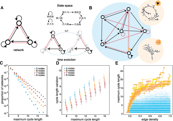
Figure 1.

Boolean network model. (A)(left) Example of an interaction network. Red indicates an inhibitory connection; black indicates an excitatory connection. Curved arrows indicate self-loops. (A)(bottom, right) Two consecutive temporal states of the network on the left. Connections not in use are shown in grey. The state of each node is shown as a ‘0’ or ‘1’ inside the relevant circle. (A)(top, right) The full state space of the network is shown on the left. Arrows indicate the temporal progression from state to state. Each state is encoded as the activity of the three nodes (e.g. ‘(0,1,1)’ listed clockwise starting from the top one). (B) A larger interaction network of 56 nodes. The state space of this network will depend upon whether the orange edge is excitatory or inhibitory. In the former case, the state space is as shown in the top beige circle; in the latter case, the state space is as shown in the bottom beige circle. (C) Distribution of maximum cycle length for uniformly sampled networks of 5, 6, 7, and 8. (D) Expected decrement in cycle length (x-axis) when a single edge is randomly altered (y-axis). (E) Optimized networks for cycle length obtained by random sampling (blue) and by a Pareto evolutionary algorithm (orange).