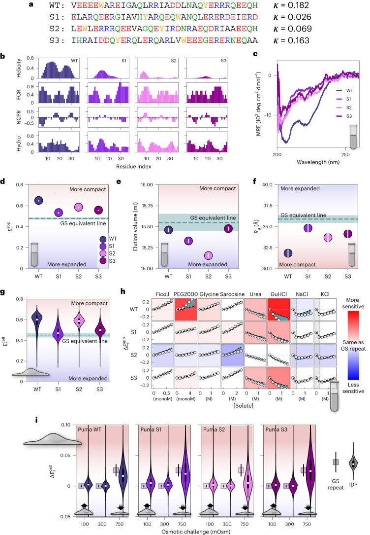
Fig. 3. Sequence-dependent structural biases of PUMA BH3 domain.
a, Sequence of WT PUMA BH3 domain and three sequences (S1, S2 and S3) derived by shuffling WT PUMA’s sequence. κ measures clustering of charged residues in the sequence, with a value closer to 1 for sequences where like charges are highly clustered. b, Molecular features of PUMA sequences. FCR, fraction of charged residues; NCPR, net charge per residue; Hydro: Kyte–Doolittle hydrophobicity. Values are the average of the five nearest residues. c, CD spectroscopy of PUMA variants without flanking FPs. See also Supplementary Fig. 9. d, Average of PUMA constructs. Error bars represent the standard deviation (N = 12), the teal dashed line is the interpolated value for a 34-residue GS repeat, and the shaded teal area is the error from the interpolation. Blue/red shading indicates expansion/compaction compared to GS repeat. e, SEC elution volume for PUMA constructs. Errors are obtained from determination of peak position in Supplementary Fig. 2. Teal dashed line and blue/red shading as in d. f, SAXS-derived Rg of PUMA constructs. Error bars are calculated from linear fits to Guinier plots (Supplementary Fig. 3). Teal dashed line and blue/red shading as in d. g, of PUMA constructs. Features are as in Fig. 2g. Teal dashed line and blue/red shading as in d. h, of PUMA constructs in response to solution changes. Black dashed lines are interpolated of a GS repeat sequence of the same length as the IDP (Supplementary Fig. 12). Green shaded regions are differences between of IDP and GS repeats. Gray error bars indicate the spread of the data over two repeats. The background color for each plot indicates the sensitivity of the IDP to that solute, with red/blue being more/less sensitive (compared to the GS repeat). i, of PUMA constructs (violins) and GS repeat equivalents (squares). Features are as in Fig. 2g. The dataset used to generate all live cell figures is in Supplementary Data 3. N for each violin plot is in Supplementary Data 4.

