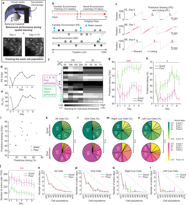
Fig. 2. Behavioral performance of mice and dynamics of the active neural ensemble of the MEC during spatial learning in virtual reality.

a Experiment schematic. An example FOV of calcium imaging indicates reliable cell tracking across days (blue arrows). Scale bar: 50 µm. Diagram is adapted from Gu et al.^33,94. b Task schematic. c Behavioral examples of mice in FE on day 0 (top) and in NE on day 1 (middle) and day 4 (bottom). Black arrows indicate the locations near rewards where predictive slowing (PS) and licking (PL) occurred. d–e Example of PS (d) and PL (e) of one mouse. f Ranking of the 15 mice under four distance thresholds for PS and PL. g–h PS under 150 cm threshold (g) and PL under 20 cm threshold (h) of good and poor performers, as in all following figures. Significance is expected because the two groups were defined using a combination of the same criteria (PS and PL) that were used for statistical testing. i Correlation between averaged PS and PL over 10 days in the NE. j Number of active cells per FOV. k–n Fractions of all cells (k), grid cells (l), right cue cells (m), and left cue cells (n) active on different days. o–r Number of days the individual cell populations in (k–n) stayed active during the 11 days (o – all cells; p – grid cells; q – right cue cells; r – left cue cells). Gray dashed lines represent the maximum number of days a cell could be active based on the first day identified. *p ≤ 0.05, **p ≤ 0.01, ***p ≤ 0.001. Error bars represent mean ± sem. Horizontal gray lines indicate p values for the group difference. See Supplementary Data 1 for exact n and detailed statistical information. Source data are provided as a Source Data file. See also Figs. S1 and S2.