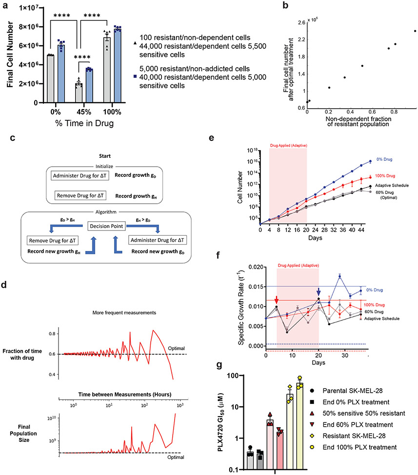
Fig 5: Optimal scheduling can be approximated with a mixed cell population of unknown growth rates.

a, A mixture of the specified ratios of UACC62 cells were treated with 1 μM PLX4720 at the indicated schedules 24 hours later. Cells were counted on day 9. One-way ANOVA with Tukey’s multiple-comparison test. p-values; **** <0.0001. The data represent six independent experiments (n =6) b, Using empirically constrained simulations, we plot the total population count as the fraction of non-dependent resistant cells varying from 0% to 100% of the resistant population. c, A cartoon schematic of the blind adaptive therapy algorithm. d, (Top) Using empirically measured growth rates, we simulate the fraction of time spent exposed to a drug following the blind adaptive therapy (solid red line) and compare it to the true optimal (dotted black line) as a function of how frequently population-level growth rates can be measured. (Bottom) The same simulations as above but now showing the final cell count of the population (solid red line) is compared to what is projected from the optimal schedule (black dotted line). e, Results of the blind adaptive therapy experiment. Cell counts over time were recorded, and the shaded red region highlights the time the drug was applied. f, Growth rates for each schedule at the indicated time points. The growth rate of parental SKMEL28 cells in DMSO (solid blue line) and BRAFi (blue dashed line) is indicated. Arrows indicate time points when the treatment condition was changed due to the measurement. The growth rate of PLX-resistant pooled SKMEL28 cells in 1 μM PLX4720 (solid red line), and DMSO (red dashed line) is indicated. The red region highlights the period the drug was applied. g, The PLX4720 GI₅₀ values of the ending cell populations in e compared to the PLX4720 GI₅₀ values of the indicated known mixtures of parental and resistant SKMEL28 cells. e, g, These data represent three independent experiments (n =3). a, e-g, Data are presented as mean ± SEM.