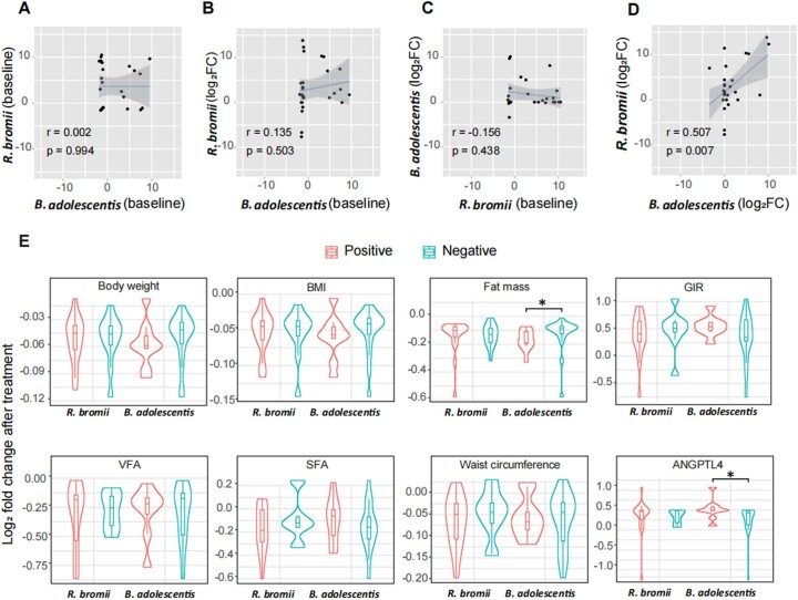
Extended Data Fig. 4. Baseline abundances of two primary degrading microbiota of RS and their relationship with clinical outcomes.
(a-d) The two-tailed Pearson correlation between (a) the baseline abundances of B. adolescentis and R. bromii. (b) the baseline abundances of B. adolescentis and the abundance change of R. bromii. (c) the baseline abundances of R. bromii and the abundance change of B. adolescentis. (d) the abundance changes of B. adolescentis and R. bromii. The changes in B. adolescentis and R. bromii are calculated by the log2 fold change after treatment. Baseline abundance values have undergone centred log-ratio (CLR) transformation before correlation analysis. The lines and grey zones show the fitted linear regression lines with 95% confidence intervals. (e) The relationship between the presence of key species (B. adolescentis and R. bromii) and the change of key outcomes after RS treatment. The changes of key outcomes were presented by the log2 fold change after treatment. The violin plots illustrate the kernel density estimation of the data distribution, and the embedded box plots indicate the median and interquartile range. Whiskers extend to 1.5 times the IQR. n = 16 for R. bromii positive individuals, n = 11 for R. bromii negative individuals, n = 9 for B. adolescentis positive individuals, and n = 18 for B. adolescentis negative individuals. Statistical differences between the positive and negative groups were assessed using the two-sided Wilcoxon rank-sum test, with P values displayed above the plots. * P = 0.033 and 0.046 for fat mass and ANGPTL4 (e). The colour indicates the presence (positive, orange) or absence (negative, cyan) of key species.

