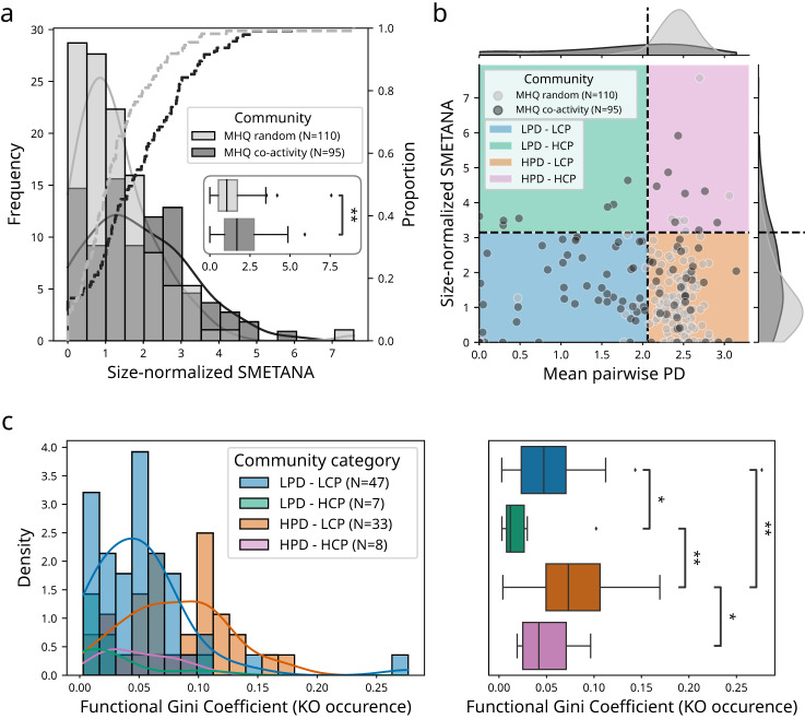
Fig. 4. Community-wide metabolic modelling reveals a higher metabolic interaction potential within marine prokaryotic communities.

a Microbial communities were delineated on the global co-active genome network using the MCL graph clustering algorithm (see “Methods”). Community metabolic modelling was performed using SMETANA on co-active communities (N = 95, dark grey, frequencies as bars and proportions as dashed line) and compared to random communities (N = 110, light grey). Boxplot insert: Co-active communities (dark grey) overall displayed a significantly higher metabolic interaction potential (SMETANA) score as compared with random communities (Mann–Whitney U test two-sided, p = 1.09 × 10 ^− 3). b Distinct metabolic interactions community types were identified within co-active marine prokaryotic communities (black points) and differentiated from random communities (grey points), the latter largely displaying an overall higher mean phylogenetic distance and lower metabolic cross-feeding potential score (HPD-LCP, orange quadrant): (i) Communities with overall low mean phylogenetic distance and low metabolic cross-feeding potential score (LPD-LCP, blue quadrant), (ii) communities with overall low mean phylogenetic distance and high metabolic cross-feeding potential score (LPD-HCP, green quadrant), and (iii) communities with overall high mean phylogenetic distance and high metabolic cross-feeding potential score (HPD-HCP, pink quadrant). LPD co-active communities had a mean phylogenetic distance smaller than 95% of the random communities, while HCP have a mean SMETANA score above 95% of the random communities (dotted black lines). c HPD communities (orange N = 33, and pink N = 8) were more dissimilar to respective LPD communities (blue N = 47, and green N = 7) according to their functional Gini coefficient inferred from KEGG metabolism KO genes occurrence profiles (Mann–Whitney U test two-sided with Benjamini-Hochberg correction, LPD-LCP vs. LPD-HCP p = 4.88 × 10 ^− 2, LPD-HCP vs. HPD-LCP p = 2.77 × 10 ^− 3, HPD-LCP vs. HPD–HCP p = 4.89 × 10 ^− 2, LPD-LCP vs. HPD-LCP p = 1.30 × 10⁻³). The box extends from the lower to upper quartile values of the data (Q1 and Q3), with a line at the median (Q2). The whiskers extend from the box to show the range of the data and are defined as follows: where IQR is the interquartile range (Q3-Q1), the upper whisker will extend to last data point less than Q3 + 1.5 × IQR. Similarly, the lower whisker will extend to the first data point greater than Q1–1.5 × IQR. Beyond the whiskers, data are plotted as individual points.