Single proxy control

ABSTRACT

Negative control variables are sometimes used in nonexperimental studies to detect the presence of confounding by hidden factors. A negative control outcome (NCO) is an outcome that is influenced by unobserved confounders of the exposure effects on the outcome in view, but is not causally impacted by the exposure. Tchetgen Tchetgen (2013) introduced the Control Outcome Calibration Approach (COCA) as a formal NCO counterfactual method to detect and correct for residual confounding bias. For identification, COCA treats the NCO as an error-prone proxy of the treatment-free counterfactual outcome of interest, and involves regressing the NCO on the treatment-free counterfactual, together with a rank-preserving structural model, which assumes a constant individual-level causal effect. In this work, we establish nonparametric COCA identification for the average causal effect for the treated, without requiring rank-preservation, therefore accommodating unrestricted effect heterogeneity across units. This nonparametric identification result has important practical implications, as it provides single-proxy confounding control, in contrast to recently proposed proximal causal inference, which relies for identification on a pair of confounding proxies. For COCA estimation we propose 3 separate strategies: (i) an extended propensity score approach, (ii) an outcome bridge function approach, and (iii) a doubly-robust approach. Finally, we illustrate the proposed methods in an application evaluating the causal impact of a Zika virus outbreak on birth rate in Brazil.

1. INTRODUCTION

Unmeasured confounding is a well-known threat to valid causal inference from observational data. An approach that is sometimes used in practice to assess residual confounding bias, is to check whether known null effects can be recovered free of bias, by evaluating whether the exposure or treatment of interest is found to be associated with a so-called negative control outcome (NCO), upon adjusting for measured confounders (Rosenbaum, 1989; Lipsitch et al., 2010; Shi et al., 2020). An observed variable is said to be a valid NCO or more broadly, an outcome confounding proxy, to the extent that it is associated with hidden factors confounding the exposure-outcome relationship in view, although not directly impacted by the exposure. Therefore, an NCO that is empirically associated with the exposure, might suggest the presence of residual confounding. In the event such an association is present, a natural question is whether the NCO can be used for bias correction.

The most well-established NCO approach for debiasing observational causal effect estimates is the difference-in-differences approach (DiD) (Card and Krueger, 1994; Lechner, 2011; Caniglia and Murray, 2020). In fact, DiD may be viewed as directly leveraging the pretreatment outcome as an NCO since it cannot logically be causally impacted by the treatment. Identification then follows from an additive equi-confounding assumption that the unmeasured confounder association with the post-treatment outcome of interest matches that with the pre-treatment outcome on the additive scale (Sofer et al., 2016). The baseline outcome in DiD is thus implicitly assumed to be a valid NCO, and equi-confounding is equivalent to the so-called parallel trends assumption, that the average trends in treatment-free potential outcomes for treatment and untreated units are parallel. In practice, equi-confounding or equivalently parallel trends may not be reasonable for a number of reasons, including if the outcome trend is also impacted by an unmeasured common cause with the treatment. Furthermore, additive equi-confounding may not be realistic as a broader debiasing method in non-DiD settings where the NCO is not necessarily a pre-treatment measurement of the outcome of interest, but is instead a post-treatment measurement of a different type of outcome (and might therefore have support on a different scale than the outcome of interest has).

To address these potential limitations of additive equi-confounding, Tchetgen Tchetgen (2013) introduced the Control Outcome Calibration Approach (COCA) as a simple yet formal counterfactual NCO approach to debias causal effect estimates in observational analyses. At its core, COCA essentially treats the NCO variable as a proxy measurement for the treatment-free potential outcome, which therefore is associated with the latter, and which becomes independent of the treatment assignment mechanism, upon conditioning on the treatment-free counterfactual outcome. As the treatment-free potential outcome can be viewed as an ultimate source of unmeasured confounding, this assumption formalizes the idea that, as a relevant proxy for the source of residual confounding, the NCO would be made irrelevant for the treatment assignment mechanism if one were to hypothetically condition on the underlying potential outcome.

For identification and inference for a continuous outcome, the original COCA approach of Tchetgen Tchetgen (2013) involves the correct specification of a regression model for the NCO, conditional on the treatment-free potential outcome and measured confounders, together with a rank-preserving structural model, which effectively assumes a constant individual-level treatment effect. In this paper, we develop a nonparametric COCA identification framework for the average causal effect for the treated, which equally applies irrespective of the nature of the primary outcome, whether binary, continuous, or polytomous. Importantly, as we show, the proposed COCA identification framework completely obviates the need for rank preservation, therefore accommodating an arbitrary degree of effect heterogeneity across units. Relatedly, an alternative counterfactual approach named proximal causal inference has recently developed in causal inference literature (Miao et al., 2016; 2018; Tchetgen Tchetgen et al., 2024), which leverages a pair of negative treatment and outcome control variables, or more broadly treatment and outcome confounding proxies, to nonparametrically identify treatment causal effects subject to residual confounding without invoking a rank-preservation assumption. Importantly, while proximal causal inference relies on 2 proxies for causal identification, in contrast, COCA is a single-proxy control approach, which therefore may present practical advantages. For estimation and inference, we introduce three strategies to implement COCA, which improve on prior methods: (i) an extended propensity score (EPS) approach, (ii) a so-called outcome calibration bridge function approach, and (iii) a doubly robust approach, which carefully combines approaches (i) and (ii) and remains unbiased, provided that either approach is also unbiased, without necessarily knowing, which method might not be unbiased. Finally, we illustrate the methods with an application evaluating the causal effect of a Zika outbreak on birth rate in Brazil, and we conclude with possible extensions to our methods and a brief discussion.

2. NOTATION AND BRIEF REVIEW OF COCA

Consider an observational study where, as represented in Figure 1, one has observed an outcome variable Y, a binary treatment A whose causal effect on Y is of interest, and measured pretreatment covariates X. We are concerned that as displayed succinctly in the figure with the bow arc, the association between A and Y is confounded by hidden factors.

FIGURE 1.

A Graphical Illustration of a simple causal model.

Throughout, Y^a denotes the potential outcome or counterfactual, had possibly contrary to fact, the exposure been set to by an external hypothetical intervention. Furthermore, throughout, we also make the consistency assumption:

Assumption 1

Y = Y^A almost surely.

Hereafter, we aim to make inferences about the causal effect of treatment on the treated (ETT), denoted by . Under consistency, 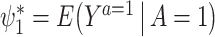is identified by ; to identify the counterfactual mean requires additional assumptions. Standard methods often resort to the no unmeasured confounding assumption, that is, , a strong assumption we do not make. Instead, we suppose that one has measured a valid NCO W, possibly multidimensional, which is known a priori to satisfy the following conditions:

Assumption 2

Condition (i): W^a = W almost surely for a = 0, 1, where W^a is the potential NCO under an external intervention that sets A = a; condition (ii): ; condition (iii): .

Assumption 2-(i) encodes the key assumption of a known null causal effect of the treatment on the NCO in potential outcome notation. Assumption 2-(ii) encodes that W is relevant for predicting the treatment-free potential outcome of interest. Assumption 2-(iii) states that W is independent of A conditional on treatment-free potential outcome and covariates. These conditions formally encode the assumption that W is a valid proxy for the treatment-free potential outcome, a source of residual confounding bias; W is only associated with the treatment mechanism to the extent that it is associated with the confounding mechanism captured by the potential outcome. We illustrate these NCO assumptions with the causal graph displayed in Figure 2. The thick arrows in the graph indicate the deterministic relationship defining the observed outcome in terms of potential outcomes and treatment variables by the consistency assumption. The missing arrows on the graph formally encode the core conditional independence conditions implied by Assumption 2.

FIGURE 2.

A graphical illustration of the assumptions for COCA. Thick arrows depict the deterministic relationship between Y and , as established by the consistency assumption (Assumption 1).

It is instructive to consider a data generating mechanism that is compatible with Assumption 2. As an example, we consider the following latent variable model for a continuous outcome:

(1a)

(1b)

where U is a continuously distributed unobserved variable and h_y(u, x) is a function that is strictly monotone in u for all x, but otherwise completely unrestricted. In the Supplementary Material A.1, we establish that expressions (1a-b) imply Assumption 2. Expression (1a) means that the treatment-free outcome is a monotonic transformation of an unobserved variable U₀, a specific instance of a so-called changes-in-changes model (Athey and Imbens, 2006). Although the latter would also assume under the causal graph in Figure 2 that W = h_w(U₀, X) where h_w(u, x) is strictly monotone in u for all x, an assumption we do not make. Expression (1b) corresponds to Assumption 2-(ii) and (iii). In fact, our formulation accommodates an additional measurement error in W, say ϵ_w, so that W = h_w(U₀, X, ϵ_w) where h_w(u, x, ϵ_w) varies in u (potentially non-monotonic) and , (1b) is satisfied. Figure 3 provides a graphical representation compatible with, although not necessarily with, expressions (1a-b).

FIGURE 3.

A graphical illustration of a structural model compatible with (1). Measured covariates X are suppressed for simplicity. The thick arrows depict the deterministic relationships Y^{a = 0} = h_y(U₀) and Y = Y^A.

For identification and estimation in the case of a continuous outcome, Tchetgen Tchetgen (2013) further assumed the rank-preserving structural model:

(2)

which, by consistency, implies a constant individual-level causal effect ψ* = Y^{a = 1} − Y^{a = 0}. Under this model, he noted that upon defining Y(ψ) = Y − ψA, then one can deduce from Assumption 2 that if and only if ψ = ψ*, in which case, given (2), Y^{a = 0} = Y(ψ*) = Y − ψ*A, which motivates a regression-based implementation of COCA, that entails searching for the parameter value of ψ = ψ* such that . A straightforward implementation of the approach uses linear models whereby for each value of ψ on a sufficiently fine grid, one obtains an estimate of the regression model using ordinary least squares (OLS), with estimated coefficients . Then a 95% confidence interval (CI) for ψ* consists of all values of ψ for which a valid test of the null hypothesis β₂(ψ) = 0 fails to reject at the 0.05 type 1 error level. Such hypothesis test might be performed by verifying whether the interval covers 0, with the OLS estimate of the standard error of . Tchetgen Tchetgen (2013) also describes a potentially simpler one-shot approach, which fits a single regression via OLS where in which case where are OLS estimates; a corresponding standard error estimator of is given in the Supplementary Material A.2 for convenience. Though practically convenient, validity of either approach relies on both correct specification of the linear model for W given (Y^{a = 0}, X), and on the rank-preserving structural model, which may be biologically implausible. In the following, we describe alternative methods aimed at addressing these limitations.

3. IDENTIFICATION OF THE EFFECT OF TREATMENT ON THE TREATED

3.1. Identification via EPS weighting

In order to establish identification, consider the EPS function:

which makes explicit the fact that, in the presence of unmeasured confounding, the treatment mechanism will generally depend on the treatment-free potential outcome even after conditioning for all observed confounders. For notational brevity, we denote the treatment odds by ω*(y, x) = π*(y, x)/{1 − π*(y, x)}. Since ω* and π* have a one-to-one relationship, we use ω* throughout to model the exposure mechanism. We assume that positivity holds, that is,

Assumption 3

where is the support of for a = 0, 1.

Next, we note that were ω* known, the average treatment-free potential outcome in the treated would then be empirically identified by the expression

(3)

See the Supplementary Material B.1 for the details. Therefore, the ETT would be identified by

As ω* is unknown, we next demonstrate how the NCO assumption can be leveraged to identify the latter quantity. Let . The proposed approach to identify ω* is based on the following equality, which we prove in the Supplementary Material B.2:

Result 1

Under Assumptions 1-3, the following result holds almost surely:

(4)

where is the conditional law of Y given (W, X, A) evaluated at Y = y, and in slight abuse of notation, may be interpreted as an integral for continuous .

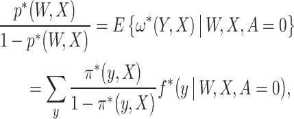
Result 1 provides an expression relating the exposure mechanism of interest to the observed data distribution, as of the 3 quantities involved in the expression p*, f*, and ω*; 2 are uniquely determined by the observed data, mainly p* and f*, which are then related to the unknown function of interest ω* in result 1; see the Supplementary Material A.3 for a graphical illustration. Equation (4) is known as an integral equation, more precisely a Fredholm integral equation of the first kind. In slight abuse of notation, the sum may be interpreted as an integral if Y is Lebesgue measurable. We then have the following identification result.

Result 2

If Assumptions 1-3 hold, and the integral equation (4) in result 1 admits a unique solution, then ω* and π* are nonparametrically identified from the observed data by solving (4), and is nonparametrically identified by (3).

Sufficient conditions for the existence and uniqueness of a solution to such an equation are well-studied; see the Supplementary Material A.5 for details. Such conditions were recently discussed in the context of proximal causal inference (Miao et al., 2016; 2018; Tchetgen Tchetgen et al., 2024). A detailed comparison of COCA with proximal causal inference is relegated to Section 6. Intuitively, the condition that the integral equation admits a unique solution essentially requires that W is sufficiently relevant for Y^{a = 0} in the sense that for any variation in the latter, there is corresponding variation in the former. This assumption is akin to the assumption of relevance in the context of instrumental variable methodology, which states that variation in the instrument should induce variation in the treatment. Importantly, Result 2 applies whether Y is binary, continuous or polytomous, provided that W is sufficiently relevant for Y^{a = 0}, to ensure that equation (3) admits a solution. Also, the result obviates the need for a rank-preserving structural model, and delivers fully nonparametric identification of the causal effect of treatment on the treated.

3.2. Identification via COCA confounding bridge function

In this Section, we introduce an alternative nonparametric identification and estimation approach, which does not rely on modeling the EPS, but instead relies on the existence of a so-called confounding bridge function formalized below.

Assumption 4

For all (y, x), there exists a function (possibly nonlinear) b*(w, x) that satisfies the following equation

(5)

Intuitively, upon noting that under Assumptions 1-2, Assumption 4 can equivalently be stated in terms of potential outcomes

(6)

which essentially formalizes the idea that W is a sufficiently relevant proxy for the potential outcome Y^{a = 0} if there exist a (potentially nonlinear) transformation of (W, X) whose conditional expectation given (Y^{a = 0}, X) recovers Y^{a = 0}. As b*(W, X) provides a bridge between the observed data equation (5), and its potential outcome counterpart (6), we aptly refer to b*(W, X) as a COCA confounding bridge function. Note that classical measurement error is a special case of the equation in the display above in which case b* is the identity map and W = Y^{a = 0} + e where e is an independent mean zero error. The condition can therefore be viewed as a nonparametric generalization of classical measurement error which allows W and Y to be of arbitrary nature and does not assume the error to be unbiased on the additive scale. We further illustrate the assumption in the case of binary W and Y. As shown in the Supplementary Material B.4, in this case with suppressing covariates, the following b*(W) satisfies (5):

provided that , encoding the requirement that W cannot be independent of Y^{a = 0}, i.e., Assumption 2. Beyond the binary case, for more general outcome types, Assumption 4 likewise formally defines a Fredholm integral equation of the first kind, for which sufficient conditions for existence of a solution are well characterized in functional analysis textbooks; we again refer the reader to Miao et al. (2016) and the Supplementary Material A.5. We are now ready to state our result, which we prove in the Supplementary  Material B.5:

Result 3

Suppose that Assumptions 1–4 hold, and b* satisfies (5). Then,

(7)

In the binary example discussed above where b*(w) was uniquely identified, we have that

We briefly highlight a key feature of the above result reflected in its proof, which is that b*(W, X) need not be uniquely identified by equation (5), and that any such solution leads to a unique value for Interestingly, the identifying formula in the display above was also obtained by Tchetgen Tchetgen (2013) in the binary case, although he did not emphasize the key role of the bridge function as a general framework for identification beyond the binary case.

3.3. Semiparametric efficiency theory

Let denote a semiparametric model defined as a collection of observed data laws that admit a solution to (5), that is,

We further consider the following surjectivity condition:

• (Surjectivity): Let denote the operator given by . At the true data law, T is surjective.

The surjectivity condition states that the Hilbert space is sufficiently rich so that any element in can be recovered from an element in via the conditional expectation mapping; see Cui et al. (2023), Dukes et al. (2023), and Ying et al. (2023) for related discussions. In addition, we consider a submodel :

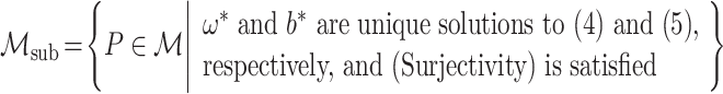We then establish the semiparametric local efficiency bound for ψ* under at the submodel .

Result 4

Suppose that Assumptions 1-4 hold. Then, the following results hold.

• The following function is an influence function for ψ* under .

  (8)

• The influence function is the efficient influence function for ψ* under at the submodel . Therefore, the corresponding semiparametric local efficiency bound for ψ* is .

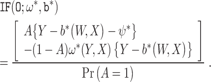
The influence function shares similarity with an influence function for ψ* in the proximal causal inference framework; see Section G of Cui et al. (2023) for details. Interestingly, the influence function has the following doubly robust property (Scharfstein et al., 1999; Bang and Robins, 2005); see the Supplementary Material B.6 for the proof:

Result 5

Suppose that Assumptions 1-4 are satisfied. In addition, suppose that either (i) or (ii) ω^†(y, x) = ω*(y, x), but not necessarily both, is satisfied. Then, we have that .

In words, if either the COCA confounding bridge function or the EPS, but not necessarily both, is correctly specified, the influence function is an unbiased estimating function of ψ*.

Using expressions (3), (7), and (8), one can construct parametric estimators of ψ*. Specifically, the first estimator using (3) entails a priori specifying a parametric model for the EPS, say a logistic regression model. The second estimator based on (7) entails a priori specifying a parametric model for the COCA bridge function, say a linear model. Lastly, the third estimator based on (8) entails parametric models for both EPS and COCA bridge functions. The first two estimators rely on the correct exposure and COCA bridge function specifications, respectively. Thus, misspecification of either model will likely result in biased inferences about the ETT. On the other hand, the last estimator has a doubly-robust property (Scharfstein et al., 1999; Bang and Robins, 2005) in that it can be used for unbiased inference about the ETT if either EPS or COCA bridge function is correct, without a priori knowledge of which model, if any, is incorrect. In the Supplementary Material A.4, we provide details on constructing these 3 parametric estimators and their large sample behavior.

A significant limitation of the three parametric estimators is their dependence on specific parametric specifications of nuisance components, which can lead to biased inference if the model specifications are incorrect. To address this concern, a potential solution is to develop an estimator where nuisance components are estimated using nonparametric methods, drawing on advancements in recent learning theory. In the following Section, we construct such an estimator and study its statistical properties.

4. A SEMIPARAMETRIC LOCALLY EFFICIENT ESTIMATOR

Our estimator is derived from the influence function in Result 5 and adopts the cross-fitting approach (Schick, 1986; Chernozhukov et al., 2018), which is implemented as follows. We randomly split N study units, denoted by 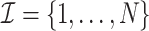, into K non-overlapping folds, denoted by . For each k = 1, …, K, we estimate the EPS and COCA confounding bridge functions using observations in , and then evaluate the estimated nuisance functions using observations in to obtain an estimator of ψ*. We refer to and as the estimation and evaluation folds, respectively. To use the entire sample, we take the simple average of the K estimators.

We introduce the following additional notation in order to facilitate the discussion. Let be the Reproducing Kernel Hilbert Space (RKHS) of V endowed with a universal kernel function , such as the Gaussian kernel , i.e., where κ ∈ (0, ∞) is a bandwidth parameter; see Chapter 4 of Steinwart and Christmann (2008) for the definition and examples of the universal kernal function. For each k = 1, …, K, let and . For a function g(O), let ‖g‖_{P, 2} = [E{g²(O)}]^1/2 be the L₂(P)-norm of g.

We estimate the EPS and COCA bridge functions by adopting a recently developed minimax estimation approach (Ghassami et al., 2022). We remark that other approaches (eg, Mastouri et al. (2021)) can also be adopted with minor modification. Note that ω*(Y, X) and b*(W, X) satisfy

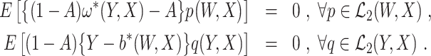Therefore, following Ghassami et al. (2022), minimax estimators of ω* and b* are given by

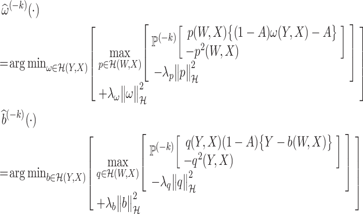where is an RKHS norm and λ_p, λ_ω, λ_q, and λ_b are positive regularization parameters.

We make a few remarks about the minimax estimation approach, of which details are relegated to Section A.6 of the Supplementary Material. First, despite the complicated formulas, closed-form representations of and are available from the representer theorem (Kimeldorf and Wahba, 1970; Schölkopf et al., 2001). Second, the bandwidth and regularization parameters can be selected via cross-validation. Lastly, ω* may vary widely because it is a ratio of 2 probabilities. In such cases, the proposed minimax estimator may result in significantly small or negative estimates. To mitigate this issue, one may consider a practical approach to regularize the minimax estimator when it appears to be ill-behaved.

Using the minimax estimators of the nuisance functions, a semiparametric estimator of ψ* is then obtained as follows:

Under regularity conditions, the semiparametric estimator is consistent and asymptotically normal for ψ*.

Assumption 5

Suppose that the following conditions hold for all k = 1, …, K:

• (Boundedness) There exists a finite constant C > 0 such that

  

• (Consistency) As N → ∞, we have and .

• (Cross-product rates) As N → ∞, we have

  

Assumption 5-(i) states that nuisance functions and the corresponding estimators are uniformly bounded. Assumption 5-(ii) states that the estimated nuisance functions are consistent for the true nuisance functions in the L₂(P) norm sense. Assumption 5-(iii) states that the cross-product rate of nuisance function estimators are o_P(N^−1/2). Assumption 5-(iii) is satisfied if b* and ω* are sufficiently smooth, the conditional expectation operators and are sufficiently smooth, and and are estimated over an RKHS with fast enough eigendecay; see Section 5 of Ghassami et al. (2022) for details. Importantly, if one nuisance function is estimated at sufficiently fast rates, the other nuisance function is allowed to converge at a substantially slower rate provided that the cross-products remain o_P(N^−1/2). This is an instance of the mixed-bias property described by Rotnitzky et al. (2020) and Ghassami et al. (2022). It is also worth highlighting the structure of the mixed bias in the current context which is the minimum of two product biases, each containing a bias term for a nuisance function and a projected bias term for the other nuisance function; this property was first reported in Ghassami et al. (2022) for a large class of functionals including ours.

Result 6 establishes that is consistent and asymptotically normal (CAN) for ψ*.

Result 6

Suppose that Assumptions 1-5 hold. Then, we have where , and a consistent estimator of σ² is where

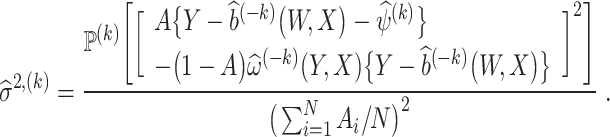
Using the variance estimator , valid 100(1 − α)% CIs for the ETT are given by where z_α is the 100αth percentile of the standard normal distribution. Alternatively, one may construct CIs using the multiplier bootstrap (van der Vaart and Wellner, 1996, Chapter 2.9); see Section A.6 for details.

Lastly, the cross-fitting estimator depends on a specific sample split, and thus, may produce outlying estimates if some split samples do not represent the entire data. To mitigate this issue, Chernozhukov et al. (2018) proposes to use median adjustment from multiple cross-fitting estimates; the detail can be found in the Supplementary Material A.6.

5. DATA APPLICATION: ZIKA VIRUS OUTBREAK IN BRAZIL

The Zika virus, which can be transmitted from a pregnant woman to her fetus, can cause serious brain abnormalities, including microcephaly (ie, an abnormally small head) (Rasmussen et al., 2016). Brazil is one of the countries hardest hit by the Zika virus. In particular, the outbreak in 2015 resulted in over 200 000 cases in Brazil by 2016 (Lowe et al., 2018). As a result, many prior works (Castro et al., 2018; Diaz-Quijano et al., 2018; Taddeo et al., 2022; Tchetgen Tchetgen et al., 2024) asked whether the Zika virus outbreak caused a drop in birth rates.

We re-analyzed the dataset analyzed in Taddeo et al. (2022) and Tchetgen Tchetgen et al. (2024). In the dataset, we focused on 673 municipalities in 2 states of Brazil, Pernambuco and Rio Grande do Sul, which are northeastern and southernmost states. Out of the 1248 cases of microcephaly that occurred in Brazil by November 28, 2015, 51.8% (646 cases) were reported in Pernambuco (PE), less than 10 cases of Zika-related microcephaly were reported in Rio Grande do Sul (RS) (Gregianini et al., 2017), which shows that PE was severely impacted by the Zika virus outbreak, while RS was minimally affected. Based on their epidemiologic histories, we defined 185 and 488 municipalities in PE and RS as treated and control groups, respectively.

For each municipality, we included the following variables in the analysis. As pre-treatment covariates, we included municipality-level population size, population density, and proportion of females measured in 2014. We used the post-epidemic municipality-level birth rate in 2016 as the outcome Y, where the birth rate is defined as the total number of live human births per 1000 persons. We used the pre-epidemic municipality-level birth rates in 2013 and 2014 as the outcome proxies (ie, NCO), denoted by W₁ and W₂, respectively. To be valid proxies, the birth rates in 2013 and 2014 must satisfy Assumption 2: (i) birth rates in 2013 and 2014 cannot be causally impacted by the Zika virus epidemic, which occurred in 2015, (ii) birth rates in 2013 and 2014 are correlated with what the birth rate in 2016 would have been had there not been a Zika virus epidemic, and (iii) birth rates in 2013 and 2014 are independent of a municipality’s Zika epidemic status, upon conditioning on its Zika virus epidemic-free potential birth rate in 2016. The first 2 conditions are uncontroversial, while the third condition largely relies on the extent to which pre-epidemic birth rates can accurately be viewed as a proxy for the counterfactual birth rate had the pandemic not occurred, and as such would not further be predictive of whether the municipality experienced a high rate of Zika virus incidence, conditional on the region’s epidemic-free counterfactual birth rate in 2016. Although one might consider this last assumption reasonable, ultimately, it is empirically untestable without making an alternative assumption. Nevertheless, in the Supplementary Material A.8, we describe a straightforward sensitivity analysis to evaluate the extent to which violation of the assumption might impact inference.

Using the dataset, we estimated , ie, the difference between the observed average birth rate of Pernambuco and a forecast of what it would have been had the Zika outbreak been prevented. Therefore, the ETT quantifies the average treatment effect (ATE) of the Zika outbreak on the birth rate within the Pernambuco region. Of note, the crude estimand was estimated to be equal to 3.384, suggesting that municipalities in the PE region (with higher incidence of Zika virus) experienced a higher birth rate than RS regions in 2016 during the Zika virus outbreak. An immediate concern is that this crude association between A and Y might be subject to significant confounding bias, leading us to conduct 2 separate analyses geared at addressing residual confounding bias; the proposed COCA methods, which we compared with a standard difference-in-differences analysis. Thus, we estimate the ETT using the approach outlined in Section 4 where the NCOs are specified as either (i) W₁, birth rate in 2013, or (ii) W₂, birth rate in 2014, or (iii) (W₁, W₂). For comparison, we also obtained doubly-robust parametric estimators of the ETT using the three NCO specifications; see the Supplementary Material A.7 for details on how these estimators were constructed.

Table 1 summarizes corresponding results. We find that the 6 COCA estimates vary between −1.833 and −2.410, meaning between 1.833 and 2.410 birth per 1000 persons were reduced in PE due to the Zika virus outbreak, an empirical finding better aligned with the scientific hypothesis that Zika may likely adversely impact the birth rates of exposed populations. Compared to the crude estimate of 3.384, the negative effect estimates indeed provide compelling evidence of potential confounding. We also obtain an estimate using the difference-in-difference estimator under a standard parallel trends assumption (eg, Card and Krueger (1994); Angrist and Pischke (2009)), which yields a considerably smaller effect estimate varying between −1.156 and −1.041; noting that the DiD estimator requires the assumption of equi-confounding of the A − Y association in the pre and postperiods, while our proposed estimator does not (but instead requires conditions (i)-(iii) outlined above). Regardless of the estimator, all estimates appear to be consistent with the anticipated adverse causal impact of the Zika Virus epidemic. Consequently, we conclude that based on inferences aimed at accounting for confounding (DiD and COCA), the Zika virus outbreak likely led to a decline in the birthrate of affected regions in Brazil, which agrees with similar findings in the literature (Castro et al., 2018; Diaz-Quijano et al., 2018; Taddeo et al., 2022; Tchetgen Tchetgen et al., 2024).

TABLE 1.

Summary of data analysis. Values in “estimate” row represent the estimates of the ETT. Values in “SE” and “95% CI” rows represent the SEs associated with the estimates and the corresponding 95% CIs, respectively.

Estimator	Statistic	NCO
		W 1	W 2	(W1, W2)
Semiparametric COCA	Estimate	−2.410	−2.182	−2.180
	SE	0.356	0.503	0.342
	95% CI	(−3.107, −1.713)	(−3.168, −1.196)	(−2.850, −1.510)
Doubly-robust parametric COCA	Estimate	−2.235	−1.833	−2.182
	SE	0.502	0.519	0.415
	95% CI	(−3.220, −1.250)	(−2.850, −0.816)	(−2.996, −1.368)
Standard DiD under parallel trends	Estimate	−1.156	−1.041	−1.041
	SE	0.199	0.195	0.195
	95% CI	(−1.546, −0.767)	(−1.424, −0.658)	(−1.424, −0.658)

The reported values are expressed as births per 1000 persons.

6. DISCUSSION AND POSSIBLE EXTENSIONS

We have described a COCA nonparametric identification framework, therefore extending previous results of Tchetgen Tchetgen (2013) to a more general setting accommodating outcomes of arbitrary nature and obviating the need for an assumption of constant treatment effects, ie, rank preservation. We have proposed 3 estimation strategies, including a doubly robust method, which has appealing robustness properties. Interestingly, the COCA central identifying assumption, that conditioning on the treatment-free counterfactual would in principle shield the treatment assignment from any association with the NCO is isomorphic to an analogous assumption in the missing data literature where an outcome might be missing not at random; however, a fully observed so-called shadow variable (the missing data analog of an NCO) reasonably assumed to be conditionally independent of the missing data process given the value of the potentially missing outcome. For example, Zahner et al. (1992) considered a study of the children’s mental health evaluated through their teachers’ assessments in Connecticut. However, the data for the teachers’ assessments are subject to nonignorable missingness. As a proxy of the teacher’s assessment, a separate parent report is available for all children in this study. The parent report is likely to be correlated with the teacher’s assessment but is unlikely to be related to the teacher’s response rate given the teacher’s assessment and fully observed covariates. Hence, the parental assessment is regarded as a shadow variable for the teacher’s assessment in this study. The literature on shadow variables is fast-growing (d’Haultfoeuille, 2010; Kott, 2014; Wang et al., 2014; Miao and Tchetgen Tchetgen, 2016; Li et al., 2023; Miao et al., 2023), the methods developed in this paper have close parallels to shadow variable counterparts in this literature. This connection to shadow variables is particularly salient when the COCA confounding bridge function is not uniquely defined, which can easily occur for instance when the shadow variable (or analogously, the NCO) is multivariate, therefore significantly complicating inference. Fortunately, the methods developed by Li et al. (2023) for the analogous shadow variable setting directly apply to the corresponding COCA setting and thus provide a complete solution for identification and inference for the ATE for the treated without relying on completeness conditions nor on unique identification of either the EPS or the COCA confounding bridge function. We refer the interested reader to this latter work for further details. It is worth noting that the doubly robust estimator proposed in this paper appears to be completely new, and different from those of Miao and Tchetgen Tchetgen (2016), Li et al. (2023), and Miao et al. (2023) and therefore may also be of use in shadow variable applications. Likewise, the doubly robust estimators proposed in the latter works can equally be applied to the current COCA setting as an alternative inferential approach.

Additionally, as mentioned in the previous section, the key assumption that conditioning on the treatment-free potential outcome would in principle make the NCO or outcome proxy irrelevant to treatment mechanism is ultimately untestable, and may in certain settings not hold exactly. In fact, this would be the case if the NCO were in fact explicitly used in assigning the treatment in which case the assumption might be violated. In order to address such eventuality, the analyst might consider several candidate proxies/NCOs when available, and may even perform an over-identification test, by inspecting the extent to which the estimated causal effect depends on the choice of proxy. Alternatively, a sensitivity analysis might also be performed to evaluate the potential impact of a hypothesized departure from the assumption. In the context of the Zika virus application, an over-identification test and a sensitivity analysis were carried out as illustrative examples, with the corresponding results and discussion provided in the Supplementary Materials A.8 and A.9.

Finally, as previously mentioned in the Introduction, COCA offers an alternative approach to proximal causal inference for debiasing observational estimates of the ETT by leveraging negative control or valid confounding proxies. A key difference highlighted earlier between these 2 frameworks is that COCA relies on a single valid NCO, which directly proxies the treatment-free potential outcome, while proximal causal inference requires both valid NCO and negative control treatment variables that proxy an underlying unmeasured confounder. Importantly, COCA takes advantage of the fact that the treatment-free potential outcome is observed in the untreated, while in proximal causal inference, the unmeasured confounders for which proxies are available, are themselves never observed, arguably a more challenging identification task. Despite the practical advantage of needing one rather than two proxies, it is important to note that though COCA identifies the ETT, it fails to nonparametrically identify the population ATE, without an additional assumption. In contrast, proximal causal inference provides nonparametric identification of both causal parameters and thus can be interpreted as providing richer identification opportunities. A key reason for this difference in the scope of identification is the fact that in the current paper, we have emphasized an interpretation of the NCO as a proxy for the treatment-free potential outcome but not for the potential outcome under treatment, in the sense that under our conditions, it must be that the treatment-free potential outcome does not only shield the treatment from the NCO, but also shields the potential outcome under treatment from the latter. Two potential strategies to recover COCA identification of the population ATE, might be either (i) evoke a rank-preservation assumption which if appropriate would imply that the ETT and the ATE are equal (this is the assumption made in Tchetgen Tchetgen (2013)); or (ii) identify a second proxy NCO which is a valid proxy for the counterfactual outcome under treatment. The second condition would be needed if Y^{a = 1} can also be viewed as a hidden confounder. By a symmetry argument, one can show that (ii) in fact would provide identification of the average counterfactual outcome under treatment for the untreated. A weighted average of both counterfactual means would then provide identification of the ATE. Details are not provided, but can easily be deduced from the presentation.

Supplementary Material

ujae027_Supplemental_Files

Web Appendices referenced in Sections 2-6 and a zip file containing the data and the analysis R code are available with this paper at the Biometrics website on Oxford Academic. The data and the analysis R code are also accessible on the GitHub repository located at http://github.com/qkrcks0218/SingleProxyControl.

FUNDING

David B. Richardson was supported by grant R01OH011409 from the National Institute for Occupational Safety and Health of the Centers for Disease Control and Prevention, and R01CA242852 from the U.S. National Cancer Institute. Eric J. Tchetgen Tchetgen was supported by NIH grants R01AI127271, R01CA222147, R01AG065276, and R01GM139926.

CONFLICT OF INTEREST

None declared.

DATA AVAILABILITY

The data and the analysis R code are accessible on Oxford Academic at the Biometrics website, as well as on the GitHub repository located at http://github.com/qkrcks0218/SingleProxyControl.

References

- Angrist J. D., Pischke J.-S. (2009). Mostly Harmless Econometrics: An Empiricist’s Companion, Princeton: Princeton University Press. [Google Scholar]
- Athey S., Imbens G. W. (2006). Identification and inference in nonlinear difference-in-differences models. Econometrica, 74, 431–497. [Google Scholar]
- Bang H., Robins J. M. (2005). Doubly robust estimation in missing data and causal inference models. Biometrics, 61, 962–973. [DOI] [PubMed] [Google Scholar]
- Caniglia E. C., Murray E. J. (2020). Difference-in-difference in the time of cholera: a gentle introduction for epidemiologists. Current Epidemiology Reports, 7, 203–211. [DOI] [PMC free article] [PubMed] [Google Scholar]
- Card D., Krueger A. B. (1994). Minimum wages and employment: A case study of the fast-food industry in New Jersey and Pennsylvania. The American Economic Review, 84, 772–793. [Google Scholar]
- Castro M. C., Han Q. C., Carvalho L. R., Victora C. G., França G. V. A. (2018). Implications of Zika virus and congenital Zika syndrome for the number of live births in Brazil. Proceedings of the National Academy of Sciences, 115, 6177–6182. [DOI] [PMC free article] [PubMed] [Google Scholar]
- Chernozhukov V., Chetverikov D., Demirer M., Duflo E., Hansen C., Newey W. et al. (2018). Double/debiased machine learning for treatment and structural parameters. The Econometrics Journal, 21, C1–C68. [Google Scholar]
- Cui Y., Pu H., Shi X., Miao W., Tchetgen Tchetgen E. (2023). Semiparametric proximal causal inference. Journal of the American Statistical Association, 1–12. [Google Scholar]
- Diaz-Quijano F. A., Pelissari D. M., Chiavegatto Filho A. D. P. (2018). Zika-associated microcephaly epidemic and birth rate reduction in Brazilian cities. American Journal of Public Health, 108, 514–516. [DOI] [PMC free article] [PubMed] [Google Scholar]
- Dukes O., Shpitser I., Tchetgen Tchetgen E. J. (2023). Proximal mediation analysis. Biometrika, 110, 973–987. [Google Scholar]
- d’Haultfoeuille X. (2010). A new instrumental method for dealing with endogenous selection. Journal of Econometrics, 154, 1–15. [Google Scholar]
- Ghassami A., Ying A., Shpitser I., Tchetgen Tchetgen E. (2022). Minimax kernel machine learning for a class of doubly robust functionals with application to proximal causal inference. In: Proceedings of The 25th International Conference on Artificial Intelligence and Statistics, vol. 151 of Proceedings of Machine Learning Research. (eds. G. Camps-Valls, F. J. R. Ruiz, and I. Valera) 7210–7239. PMLR. [Google Scholar]
- Gregianini T. S., Ranieri T., Favreto C., Nunes Z. M. A., Tumioto Giannini G. L., Sanberg N. D. et al. (2017). Emerging arboviruses in Rio Grande do Sul, Brazil: Chikungunya and Zika outbreaks, 2014-2016. Reviews in Medical Virology, 27, e1943. [DOI] [PubMed] [Google Scholar]
- Kimeldorf G. S., Wahba G. (1970). A correspondence between Bayesian estimation on stochastic processes and smoothing by splines. Annals of Mathematical Statistics, 41, 495–502. [Google Scholar]
- Kott P. S. (2014). Calibration weighting when model and calibration variables can differ. In: Contributions to sampling statistics. (eds. F. Meccati, L. P. Conti, and G. M. Ranalli) 1–18. Cambridge: Springer International Publishing, [Google Scholar]
- Lechner M. (2011). The estimation of causal effects by difference-in-difference methods. Foundations and Trends® in Econometrics, 4, 165–224. [Google Scholar]
- Li W., Miao W., Tchetgen Tchetgen E. (2023). Non-parametric inference about mean functionals of non-ignorable non-response data without identifying the joint distribution. Journal of the Royal Statistical Society Series B: Statistical Methodology, 85, 913–935. [DOI] [PMC free article] [PubMed] [Google Scholar]
- Lipsitch M., Tchetgen Tchetgen E., Cohen T. (2010). Negative controls: A tool for detecting confounding and bias in observational studies. Epidemiology, 21, 383. [DOI] [PMC free article] [PubMed] [Google Scholar]
- Lowe R., Barcellos C., Brasil P., Cruz O. G., Honório N. A., Kuper H. et al. (2018). The Zika virus epidemic in Brazil: From discovery to future implications. International Journal of Environmental Research and Public Health, 15, 96. [DOI] [PMC free article] [PubMed] [Google Scholar]
- Mastouri A., Zhu Y., Gultchin L., Korba A., Silva R., Kusner M. et al. (2021). Proximal causal learning with kernels: Two-stage estimation and moment restriction. In: Proceedings of the 38th International Conference on Machine Learning, vol. 139 of Proceedings of Machine Learning Research. (eds. M. Meila and T. Zhang) 7512–7523. PMLR. [Google Scholar]
- Miao W., Geng Z., Tchetgen Tchetgen E. (2016). Identifying causal effects with proxy variables of an unmeasured confounder. Preprint arXiv:1609.08816. [DOI] [PMC free article] [PubMed]
- Miao W., Geng Z., Tchetgen Tchetgen E. J. (2018). Identifying causal effects with proxy variables of an unmeasured confounder. Biometrika, 105, 987–993. [DOI] [PMC free article] [PubMed] [Google Scholar]
- Miao W., Liu L., Li Y., Tchetgen Tchetgen E. J., Geng Z. (2023). Identification and semiparametric efficiency theory of nonignorable missing data with a shadow variable. ACM/IMS Journal of Data Science, In press. [Google Scholar]
- Miao W., Tchetgen Tchetgen E. (2016). On varieties of doubly robust estimators under missingness not at random with a shadow variable. Biometrika, 103, 475–482. [DOI] [PMC free article] [PubMed] [Google Scholar]
- Rasmussen S. A., Jamieson D. J., Honein M. A., Petersen L. R. (2016). Zika virus and birth defects–Reviewing the evidence for causality. New England Journal of Medicine, 374, 1981–1987. [DOI] [PubMed] [Google Scholar]
- Rosenbaum P. R. (1989). The role of known effects in observational studies. Biometrics, 45, 557–569. [Google Scholar]
- Rotnitzky A., Smucler E., Robins J. M. (2020). Characterization of parameters with a mixed bias property. Biometrika, 108, 231–238. [Google Scholar]
- Scharfstein D. O., Rotnitzky A., Robins J. M. (1999). Adjusting for nonignorable drop-out using semiparametric nonresponse models. Journal of the American Statistical Association, 94, 1096–1120. [Google Scholar]
- Schick A. (1986). On asymptotically efficient estimation in semiparametric models. The Annals of Statistics, 14, 1139–1151. [Google Scholar]
- Schölkopf B., Herbrich R., Smola A. J. (2001). A generalized representer theorem. In: Computational Learning Theory. (eds. D. Helmbold and B. Williamson) 416–426. Berlin, Heidelberg: Springer. [Google Scholar]
- Shi X., Miao W., Tchetgen Tchetgen E. (2020). A selective review of negative control methods in epidemiology. Current Epidemiology Reports, 7, 190–202. [DOI] [PMC free article] [PubMed] [Google Scholar]
- Sofer T., Richardson D. B., Colicino E., Schwartz J., Tchetgen Tchetgen E. J. (2016). On negative outcome control of unobserved confounding as a generalization of difference-in-differences. Statistical Science, 31, 348–361. [DOI] [PMC free article] [PubMed] [Google Scholar]
- Steinwart I., Christmann A. (2008). Support Vector Machines, New York:Springer-Verlag [Google Scholar]
- Taddeo M. M., Amorim L. D., Aquino R. (2022). Causal measures using generalized difference-in-difference approach with nonlinear models. Statistics and Its Interface, 15, 399–413. [Google Scholar]
- Tchetgen Tchetgen E. J. (2013). The control outcome calibration approach for causal inference with unobserved confounding. American Journal of Epidemiology, 179, 633–640. [DOI] [PMC free article] [PubMed] [Google Scholar]
- Tchetgen Tchetgen E. J., Park C., Richardson D. B. (2024). Universal difference-in-differences for causal inference in epidemiology. Epidemiology, 35, 16–22. [DOI] [PMC free article] [PubMed] [Google Scholar]
- Tchetgen Tchetgen E. J., Ying A., Cui Y., Shi X., Miao W. (2024). An introduction to proximal causal inference. Statistical Science, to appear. [Google Scholar]
- van der Vaart A. W., Wellner J. A. (1996). Weak Convergence and Empirical Processes: With Applications to Statistics, New York: Springer. [Google Scholar]
- Wang S., Shao J., Kim J. K. (2014). An instrumental variable approach for identification and estimation with nonignorable nonresponse. Statistica Sinica, 24, 1097–1116. [Google Scholar]
- Ying A., Miao W., Shi X., Tchetgen Tchetgen E. J. (2023). Proximal causal inference for complex longitudinal studies. Journal of the Royal Statistical Society Series B: Statistical Methodology, 85, 684–704. [Google Scholar]
- Zahner G. E., Pawelkiewicz W., DeFrancesco J. J., Adnopoz J. (1992). Children’s mental health service needs and utilization patterns in an urban community: An epidemiological assessment. Journal of the American Academy of Child and Adolescent Psychiatry, 31, 951–960. [DOI] [PubMed] [Google Scholar]
Associated Data
This section collects any data citations, data availability statements, or supplementary materials included in this article.
Supplementary Materials