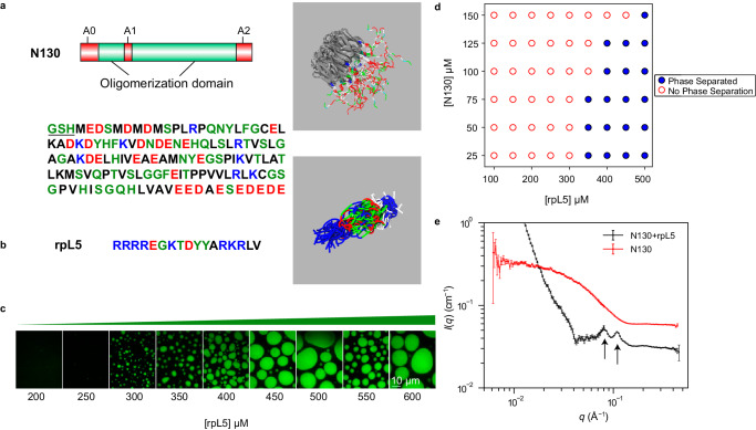
Fig. 1. Complexation between acidic regions within N130 and R-motifs of rpL5 is required for condensation.

a Schematic representation of N130 including the different acidic regions. The amino acid sequence of N130 is also shown. The three acidic regions A0, A1, and A2 span residues 4–18, 35–44, and 120–133, respectively. Non-native N-terminal residues that remain after protease cleavage are underlined. On the right, we show the overall structure of the hairy colloid generated by superposition of 50 distinct conformations from atomistic simulations. These simulations use the ABSINTH implicit solvent model⁸⁷ and explicit representations of solution ions¹³² (which are not shown in the figure). The pentamerized OD (PDB ID 4N8M), in gray, was modeled as a rigid molecule in the atomistic simulations. b The amino acid sequence of rpL5. The panel on the right shows a superposition of 50 different conformations extracted from ABSINTH-based simulations. c Confocal microscopy images of phase separation of 100 µM N130 upon titrating the concentration of rpL5 in buffer and 150 mM NaCl. N130 is labeled with AlexaFluor488. Microscopy experiments were repeated in three independent experiments with similar results. d Two-component phase boundary for N130 + rpL5, showing the result of concentration titrations. e SANS curve showing the intensity I(q) plotted against q, the scattering vector, for condensates formed by a solution of N130 (200 µM): rpL5 at 1:3 stoichiometry. Multi-peak analysis, as described by Mitrea et al.⁷¹, leads to the identification of two major peaks corresponding to 55 Å (right arrow) and 77 Å (left arrow) that are annotated on the figure. The SANS curve for N130 pentamers, in the absence of rpL5, is shown for comparison. In the interest of clarity, this curve is shifted upwards vis-à-vis the curve for the N130 + rpL5 system. We computed the scattering curve for individual N130 pentamers. These computed profiles show qualitative resemblance to the SANS curve shown here for N130 pentamers (see Supplementary Fig. 1). The error bars are propagated through each of the SANS data reduction steps, described and cited in the Methods. Intensity data are binned and circularly averaged to convert the 2D detector data into I(q) data, from which we calculate uncertainty values at each value of q. The data correspond to a single measurement ($n=1$).