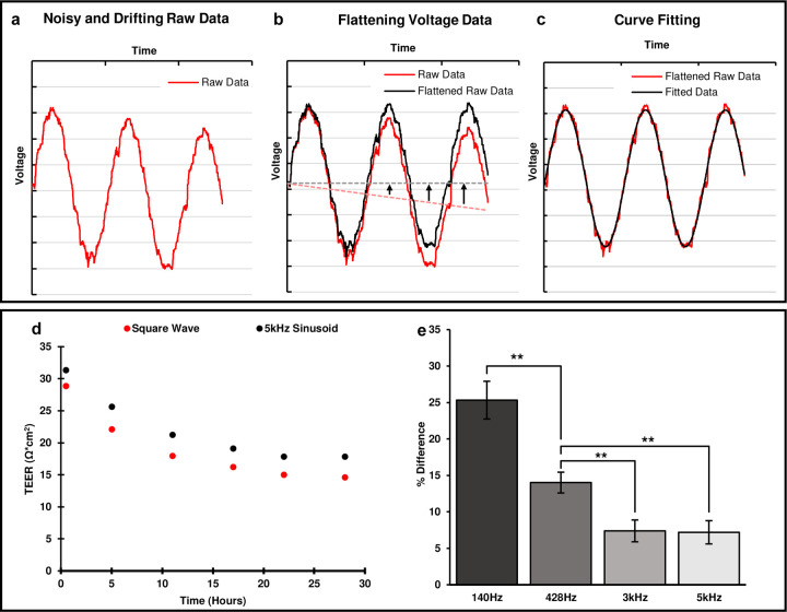
Figure 3: Response signal conditioning and the effect of stimulus signal on TEER calculation.
a) Raw response signal with unwanted artifacts. The raw data is noisy and also drifting over time because of the offset DC from the HCS. The curve-fitted signal (black) removes the unwanted artifacts from the acquired response signal (red). b) An example illustrating the drift correction performed by the fitting algorithm. The 1st degree polynomial (dotted red) of the input data is subtracted point by point from the input raw data (solid red), effectively flattening it out. Once the input data is flattened out it can be fit to a sinusoidal curve (black). c) Curve fitting algorithm applied to flattened raw data (red) to produce noise-free fitted signal (black). d) Comparison of TEER measured with square wave and 5kHz sinusoidal stimulus signals. The square wave stimulus is consistently lower than the sinusoidal value. e) The average difference of TEER between sinusoidal and square waveforms for different frequencies of the sinusoidal waveforms, n = 10, **: P < 0.005.

