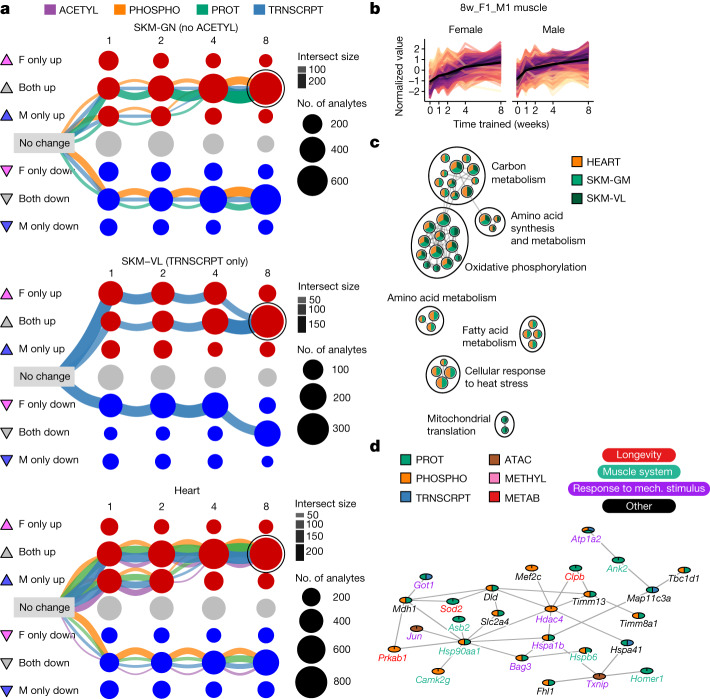
Fig. 4. Temporal patterns of the molecular training response.

a, Graphical representation of training-differential features in the three muscle tissues: gastrocnemius (SKM-GN), vastus lateralis (SKM-VL) and heart. Each node represents one of nine possible states (rows) at each of the four training time points (columns). Triangles to the left of row labels map states to symbols used in Fig. 5a. Edges represent the path of differential features over the training time course (see Extended Data Fig. 7 for a detailed explanation). Each graph includes the three largest paths of differential features in that tissue, with edges split by data type. Both node and edge size are proportional to the number of features represented. The node corresponding to features that are up-regulated in both sexes at 8 weeks of training (8w_F1_M1) is circled in each graph. b, Line plots of standardized abundances of all 8w_F1_M1 muscle features. The black line represents the average value across all features. c, Network view of significant pathway enrichment results (10% FDR) corresponding to the features in b. Nodes represent pathways; edges represent functionally similar node pairs (set similarity ≥ 0.3). Nodes are included only if they are significantly enriched in at least two of the muscle tissues, as indicated by node colour. Node size is proportional to the number of differential feature sets (for example, gastrocnemius transcripts) for which the pathway is significantly enriched. High-level biological themes were defined using Louvain community detection of the nodes. d, A subnetwork of a larger cluster identified by network clustering 8w_F1_M1 features from SKM-GN. Mech., mechanical.