RmsdXNA: RMSD prediction of nucleic acid-ligand docking poses using machine-learning method

Abstract

Small molecule drugs can be used to target nucleic acids (NA) to regulate biological processes. Computational modeling methods, such as molecular docking or scoring functions, are commonly employed to facilitate drug design. However, the accuracy of the scoring function in predicting the closest-to-native docking pose is often suboptimal. To overcome this problem, a machine learning model, RmsdXNA, was developed to predict the root-mean-square-deviation (RMSD) of ligand docking poses in NA complexes. The versatility of RmsdXNA has been demonstrated by its successful application to various complexes involving different types of NA receptors and ligands, including metal complexes and short peptides. The predicted RMSD by RmsdXNA was strongly correlated with the actual RMSD of the docked poses. RmsdXNA also outperformed the rDock scoring function in ranking and identifying closest-to-native docking poses across different structural groups and on the testing dataset. Using experimental validated results conducted on polyadenylated nuclear element for nuclear expression triplex, RmsdXNA demonstrated better screening power for the RNA-small molecule complex compared to rDock. Molecular dynamics simulations were subsequently employed to validate the binding of top-scoring ligand candidates selected by RmsdXNA and rDock on MALAT1. The results showed that RmsdXNA has a higher success rate in identifying promising ligands that can bind well to the receptor. The development of an accurate docking score for a NA–ligand complex can aid in drug discovery and development advancements. The code to use RmsdXNA is available at the GitHub repository https://github.com/laiheng001/RmsdXNA.

INTRODUCTION

Therapeutic treatments have typically focused on modifying protein targets [1, 2], but there is a growing acknowledgment of the critical role of ribonucleic acid (RNA) and deoxyribonucleic acid (DNA) molecules in numerous biological processes and disease pathways [3–6]. Dysfunctions in RNA and DNA that can cause diseases [7–9], such as cancer, neurological problems and viral infections [10, 11], can be treated using small chemicals. As our understanding of NA increases, especially with developments in computational methodologies [12, 13] and structure-solving technologies [14], targeting NA for drug development shows promise in the field of molecular medicine.

Currently, however, solving the structure of NA complexes using experimental methods remains a challenge. As an alternative, computational methods, including molecular docking, can enhance the understanding of NA complexes and expedite the development of robust drug discovery models [15–17]. Recent development of such docking tools for NA–ligand complexes includes rDock [18], NLDock [19] and RLDOCK [20]. Molecular docking involves predicting the binding orientation and affinity between a small molecule (ligand) and a target protein or NA (receptor). Its precision depends on the reliability of the scoring functions [21, 22], which is crucial for saving time and cost for drug discovery [23, 24]. However, accurate modelling of NA structures remains challenging because of its complexity and flexibility [25]. While the MM-PBSA [26] and free-energy perturbation methods [27] can accurately select stronger ligand binders compared to docking scoring functions, they are time-consuming and not suitable for high-throughput docking or virtual screening (VS) applications.

Integrating machine learning (ML) into docking algorithms can improve the accuracy and efficiency of computational tools [28–30]. Numerous ML algorithms that outperform a broad range of classical scoring functions have been successfully utilized in protein systems [31]. However, these scoring functions often cannot be applied directly to NA complexes [32, 33]. The limited availability of high-quality training datasets for NA complex structures poses a significant obstacle to the generation of accurate and robust models [34]. Hence, the exploration of alternative feature extraction and ML algorithms methods is essential for addressing these challenges.

Although not as common as protein–ligand systems, two recent ML-based scoring functions have been developed to improve scoring functions for RNA–ligand interactions. RNAPosers [35] is trained on 80 RNA–ligand complexes to classify if the ligand pose is native-like. On the other hand, AnnapuRNA [36] is trained on 131 RNA–ligand complexes to develop a scoring function for predicting binding poses. Both methods demonstrated improved performance compared to existing tools for pose identification. However, the small dataset used for training the models can lead to overfitting and hinder the model’s performance for unseen docking scenarios. In addition, both methods use interaction features involving unmodified RNA residues only, neglecting crucial interactions involving modified atoms, which can alter the chemical properties of NA [37]. A diversified model should also be applicable to some important NA–ligand complexes, such as metal complex [38] or short peptide ligands [39], and RNA–DNA hybrid receptors [40]. Developing a ML-based scoring function suitable for NAs (both DNA and RNA) and structures with modified residues seems feasible due to their structural similarity.

In this work, a new ML-based regression model, RmsdXNA, was developed for accurately predicting the RMSD of the ligand poses for NA–ligand complex, which can also serve as the docking score. Using a larger dataset of 980 PDB structures than previous studies aims to improve generalizability. As the number of NA structures is still relatively small compared to proteins, using similar distance-based fingerprints from Wang et al. [41] with small feature dimension is feasible for RmsdXNA. Further modifications to the atom representation and the machine learning algorithm were performed to better suit NA–ligand datasets. RmsdXNA is applicable to diverse complexes involving different types of NA receptors (RNA, DNA, RNA–DNA hybrid, and NA with modified residues) and ligands, including metal complexes and short peptides. The best performing RmsdXNA model achieved an average Pearson correlation coefficient (PCC) of 0.64531 0.36262 and Spearman’s rank correlation coefficient (SRCC) of 0.58465 0.35195 for each ligand. RmsdXNA outperforms the rDock [18] scoring function in its ability to rank and identify closest-to-native poses across different structural groups and on the testing dataset. This was also validated using the in-vitro experimental results by Swain et al. [42] on PAN ENE triple helix RNA. For MALAT1 virtual screening, MD simulations revealed a higher success rate for RmsdXNA in identifying the most promising ligands. These findings solidify RmsdXNA as a robust and effective scoring tool for pose identification and ligand screening in drug discovery applications.

MATERIALS AND METHODS

Dataset preparation

The dataset used in the experiments consists of experimentally solved NA structures obtained from the Nucleic Acid Database (NDB) [43, 44], which contains 11 821 NA structures including both DNA and RNA. PyMol [45] was used to process the structural information. Additional data cleaning and refinement procedures are described in Appendix B. In total, 1434 ligands from 980 NA complexes, with some structures having multiple ligands, were used in the experiment. The use of a large and diverse database allows the model to learn a comprehensive representation of the underlying patterns and relationships in the data, leading to better generalization to unseen examples. The list of PDB structures used is found in Appendix A.

Docking tools

Each ligand forms a receptor–ligand pair in each complex. Rigid NA-flexible ligand docking was performed using rDocK [18] at the target search box, with the native ligand as the reference ligand. rDock was chosen because it outperforms other docking tools in pose identification for NA complexes [19, 46]. The docking pose search algorithm of rDock is similar to that of AutoDock [47], which uses the Monte Carlo simulated annealing method to generate random poses with unique configurations in each dock attempt. This data augmentation method can mitigate the limitation of the small NA–ligand dataset by increasing the number of datapoints with generated poses. Using rDock, the rbcavity command was used to generate the docking volume, with the docking radius set to 10 Å. For each redocking run, 100 runs-per-ligand rDock jobs were performed using the rbdock command. Only the docking poses with symmetry-corrected RMSD values 10 Å, measured using sPyRMSD [48], were considered as a successful dock and were included in the training dataset. 100 poses were selected from each ligand that had at least 25% successful docking rate (able to generate at least 100 successful dock poses out of 400 dock attempts) to be included into the dataset.

Feature generation

The workflow of dataset generation and model training for RmsdXNA to predict the RMSD of the docked poses is shown in Figure 1. For each distinctive interaction between the receptor and docked ligand atoms, the interatomic distance and atom types are used as features. In the context of ML scoring functions for NAs, the quantity of structures within the dataset is notably lower than that of the proteins. Reducing the number of employed features is crucial to prevent overfitting, the curse of dimensionality and data sparsity. Previous studies such as OnionNet [49] and OnionNet2 [50] adopted the count of contact points at each shell as their feature metric, whereas RNAposers [35] employed the receptor’s atom name to generate distance-based features. However, these methodologies create an abundance of features, resulting in an unfavorable high feature-to-instance ratio dataset. On the other hand, the coarse-grain representation of the RNA and ligand structures [51, 52] in AnnapuRNA [36] might sacrifice atomic-level details, especially for non-canonical residues, potentially compromising the model’s ability to capture specific interactions.

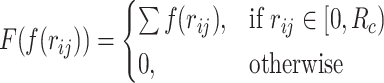
Figure 1.

Overall architecture of the RmsdXNA framework. (A) Inter-molecular distance between a NA receptor atom and the ligand atom within a cutoff distance, is extracted for each generated pose. (B) The distance is used to form the and terms, which will be concatenate with the rDock scoring components to form the features, X. The label, y is the actual RMSD of the docked poses. (C) XGBoostRegressor is used to train on the dataset predict the RMSD of the docked poses.

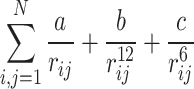
In RmsdXNA, the receptor and ligand SYBYL atom type representation is used as the interaction label. This generates fewer features in the dataset and allows the retention of important atomic-level interaction information such as pi-stacking and hydrogen bonding interactions. The remaining challenge involves combining each pairwise distance into a structured dataset suitable for training the ML model, while simultaneously retaining interaction proximity and frequency information. The distance is used to model the intermolecular potential energy between the receptor and the ligand molecule, which is represented by the sum of the coulomb and Lennard-Jones interaction terms, as shown in Equation 1. Such physics-inspired distance features were explored by Wang et al. [41] in protein–ligand interactions.

(1)

(2)

The values of the interaction constants are unknown and are factorized to form constants a, b and c. Equation 1 can be simplified to form Equation 2 by factorizing the constants. For a given receptor–ligand structure, the intermolecular distance between 2 atoms, , can be easily obtained from the structural coordinates. ML is then used to determine the arbitrary constants. Assuming that there is a correlation between the RMSD and intermolecular forces, the RMSD can be predicted using the above equations. The intuition behind this assumption is that the closer-to-native ligand pose (smaller RMSD) should have stronger intermolecular interaction with NA than other poses. For each docked ligand pose, the interaction feature values between receptor atom and ligand atom similar to Equation 2 are represented by , such that:

where:

= fingerprint function, for {, ,

} = distance between the receptor atom and ligand atom

= receptor residue-atom type, represented by

= receptor residue type, for {A, C, G, U/T, N, OTH, Metal}

= receptor SYBYL atom type

= ligand SYBYL atom type

=cutoff distance (Å), for {7, 8, 9, 10}

The NA residues can be classified into five generalized types, namely adenine (A), uracil (U) or thymine (T), cytosine (C), guanine (G), and ribose and phosphate backbone (N). The nucleobases of DNA and modified residue nucleobases are grouped into 4 main RNA nucleobases (A, U, G, C), depending on which nucleobases the residues are mutated from or have the closest structural similarity with (Appendix D), with thymine being in the same group as uracil. The NA SYBYL atom types are determined based on their position on these residues, and atoms in the backbone have residue type ’N’ (Appendix E). The atoms in the modified region of the residues have residue type ’OTH’. These NA atoms and some ligand atoms with low occurrence are grouped by their chemical similarity, as described in Appendix C. The grouping of the residues and atom types reduces the sparsity of the dataset and the number of features in the dataset by binning the columns with a high number of 0-values, hence improving the generalizability of the model and making it applicable to datasets with modified residues. In total, 24 ligand atom types and 26 NA atom types (unique combinations of the residues and its corresponding atom types) were used, resulting in 624 pairs of interactions. Subsequently, columns with all 0 values were removed from the dataset, thus a final 529 pairs of interactions were included.

In the ablation studies performed in Section 3.2, the dataset that yielded the best result used a cutoff distance, , of 8 Å, along with the combination of the 1088 and terms with the 30 rDock scoring function component terms for the features. It is noted that the model can be used to predict the RMSD of poses generated by other docking tools as the rDock scoring function components can also be obtained from the initial poses.

Machine learning models

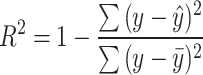
A supervised learning algorithm is used to train the ML model to predict the RMSD of docked poses, which can also be utilized as the docking score. For this regression prediction task, the XGBoost algorithm was chosen because of its fast training speed and strong predictive capabilities in comparison with other ML models such as Support Vector Regression, Multi-layer Perceptron, and Random Forest algorithms as shown in Table A4. The superior performance of XGBoost over other algorithms may be due to the sparsity of the dataset. To ensure that datasets with the same PDB ID are not present in both the training and validation datasets simultaneously, systematic sampling is employed on the sorted PDB IDs to select the validating PDB ID at regular intervals. The data points are then split into training and validation datasets by their PDB ID. For each dataset, 100 models with randomized hyperparameter values are trained using five-fold cross-validation to assess the models’ performance across different data subsets, which provides a reliable assessment of the model’s generalization capabilities. values (Equation 3) are calculated for each fold. The model with the highest average validating across all folds, , which indicates a strong correlation between predicted and actual RMSD, was selected as the best model. The model is trained with the learning objective of minimizing the regression squared loss and the hyperparameters of the best model are shown in Appendix F.

(3)

where: = Actual RMSD of pose

= Predicted RMSD of pose

= Average actual RMSD of all poses

Validation using experimental result and MD simulations

Unlike protein–ligand complexes, there is no CASF-2016 [53] equivalent dataset for evaluating NA complex docking tools. Instead, the comparison of the scoring power of RmsdXNA and rDock is validated on experimental results and using MD simulation.

In the microscale thermophoresis (MST) experiment by Swain et al. [42] on PAN triplex, Compound 15 exhibited the strongest interaction among seven hit compounds (Compounds 8, 13, 15, 18, 19, 20 and 25) identified by small-molecule microarray (SMM) screening. Weak interactions were observed for the 3 Compound 15 modifications (Compounds 15-A1, 15-A2, 15-A3) compared to Compound 15, with Compounds 15-A2 and 15-A3 failing to bind to the RNA. The structures of the compounds are shown in Figure A2. Using the MST results, an ideal docking score that can distinguish strong and weak binders should be able to accurately rank the compounds by their binding affinity and give the best ranking to Compound 15. Rigid receptor-flexible ligand docking of the compounds was performed using rDock on the dinucleotide bulge position of PAN triplex (PDB ID: 6X5N), generating 100 poses for each compound. Then, RmsdXNA and rDock scores were used to rank the compounds.

MD simulations can offer insights into the dynamic behavior of receptor–ligand complexes, thus providing a more accurate assessment of ligand trajectories stability compared to docking alone [54, 55]. In this VS example, rDock is utilized to generate 20 poses within a 20 Å target search box on the 3’ end of MALAT1 [56, 57] (PDB ID: 4PLX) against two screening compound libraries, Hit2Lead (provided by Chembridge Corp. in San Diego, CA, USA, http://www.hit2lead.com) and Life Chemicals RNA screening library (https://www.lifechemicals.com). From each library, the top 20 ligands with the best rDock and RmsdXNA scores were chosen as the top-scored ligands for each method. Then, MD simulation (described in Appendix H) was conducted on the MALAT1-top ligand complexes to assess the reliability of the docking scoring methods through visual inspection the ligands’ stability in the receptor during the 100 ns trajectory [58].

RESULTS AND DISCUSSION

Model performance

The best model obtained from the hyperparameter tuning procedure had a of 0.68301 0.02330. The predicted RMSD values of each docked ligand pose in the validation dataset were combined across all folds to obtain the overall predicted RMSD for the entire dataset. Since the validation data remain unseen by the model in each fold, the obtained predictions accurately represent the model’s generalizability. Figure 2(a) shows the comparison of the predicted RMSD with the actual RMSD of the docked poses, which has a strong correlation coefficient (R) of 0.83051 0.00115. This finding underscores the RmsdXNA’s ability to accurately predict RMSD values.

Figure 2.

Performance of RmsdXNA and its comparison with rDock on the full validation dataset.

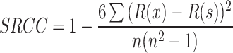
An effective score function should assign lower scores (better ranking) to the closest-to-native pose, which has a lower actual RMSD than the decoy poses. Therefore, the PCC (Equation 4) and SRCC (Equation 5) between the actual RMSD and scoring functions for each NA–ligand pair, which measure the correlations and ranking capabilities, respectively, are key metrics for evaluating their performance. Figure 2(b) and 2(c) illustrates each ligand’s distribution of the PCC and SRCC values respectively for both scoring methods. RmsdXNA has a higher average PCC and SRCC than rDock. In addition, RmsdXNA outperforms rDock for 1271/1434 (88.6%) and 1254/1434 (87.4%) ligands in terms of PCC and SRCC respectively. This comparison revealed that RmsdXNA has a stronger correlation and ranking capabilities than rDock for most of the ligand structures.

(4)

where:

= Actual RMSD of pose

= Average actual RMSD of all poses

= Score of pose

= Average score of all poses

(5)

where:

= ranking of pose based on RMSD (x)

= ranking of pose based on score (s)

= number of poses

The ability of RmsdXNA and rDock to select close-to-native poses, defined by poses with RMSD 2.0, was also analyzed. Figure 2(d) shows that the fraction of ligands that contained close-to-native poses in the top-n-scored poses was greater for RmsdXNA. Additionally, out of all the ligands that are able to generate at least 1 close-to-native pose, 69.1%, 81.9% and 86.9% of the ligands for RmsdXNA and 45.9%, 62.0% and 70.8% of the ligands for rDock contained close-to-native poses in the top 1, 5, and 10 selected poses respectively. These results showed that RmsdXNA outperforms the rDock scoring function in pose identification.

Ablation studies

Ablation experiments were conducted to investigate the impact of various modifications to dataset generation on the performance of the model. The modified dataset was used to train the model using the steps described in Section 2.4. The model with the highest for each modified dataset was subsequently selected and compared across the different modifications.

First, the effect of on dataset generation was examined and the results are summarized in Table A5. As varies from 4 to 10 Å, more interaction features are extracted and added to the dataset. New features with non-0 values may also be introduced into the dataset, increasing the number of columns of the dataset slightly. Previous studies by Szulc et al. [59] employed cutoff distances of 3.9 and 4.0 Å to detect hydrogen bonding and lipophilic interactions respectively in RNA complexes. However, = 8 Å gave the highest of 0.68301 0.02330. The improvement in the results from = 4 to 8 Å may be due to the increase in the number of non-0 values in the dataset and the addition of new information for the model. Beyond certain distances, such as = 9 and 10 Å, the added long-range and weak interaction may introduce noise to the data and additional information has insignificant contributions to the specific interaction between NA and ligand. Therefore, finding the optimal cutoff distance is vital for striking the right balance between capturing relevant interactions and avoiding unnecessary complexity in the dataset.

Next, the effect of adding the rDock scoring components, , and features into the dataset was investigated. By generating datasets that combine these specific features, their contribution to the overall model performance can be evaluated and the best performing combinations can be determined. The results of the model with different combinations of features are shown in Table A6. The best result of = 0.68301 0.02330 was achieved when the rDock scoring function components were added to the and features. The improved prediction accuracy suggests that the rDock components and the generated features complement each other effectively. Additionally, the analysis revealed that the component is less important than the and components, as the of the model decreased to 0.67910 0.01763 when the component was added to the dataset. Wang et al. [41] explained that the short-range repulsive term, , is not relevant because of the low occurrence of small-distance interactions in the NA–ligand complex. Although similar distance data are used to generate the feature values of , and , the difference in the results suggests that proper data augmentation of the feature is needed to achieve high accuracy of the model.

Finally, the impact of different atom representation methods when generating the dataset on is summarized in Table A7. The use of the SYBYL atom type to represent receptor and ligand atoms, element type to represent receptor atoms with the ’OTH’ residue type, and other grouping methods mentioned in Appendix C, achieved the highest of 0.68301 0.02330. This outperformed models that used a full element or SYBYL atom representation with values of 0.66726 0.02244 and 0.67945 0.01654 respectively. Compared to DeepRMSD, which uses element atom representation, using the SYBYL atom type can distinguish aromatic and non-aromatic atoms. This allows the model to capture pi-stacking interactions between the NA receptor and ligand which are abundant in NA complexes [60]. Additionally, to handle sparse features involving NA modified residues atoms, binning them with other meaningful features can offer more instances for the model to learn from, while reducing the introduction of biased information.

Feature importance analysis

Feature importance analysis was conducted to determine the relative importance of individual features in predicting RMSD in the model. The following training process uses the hyperparameter obtained from the best model. For each fold, the model is used to predict the RMSD of the ligands from the modified validating dataset where a specific ij pair feature ( and ), or the rDock score component is artificially removed by setting all its values to 0. The change in the performance of the model was evaluated using , which represents the difference in between the original validation dataset and the dataset with the removed columns. This process is repeated for all columns, and the features that result in a decrease in are identified as important, whereas those resulting in an increase in are considered less important. This analysis is performed for each fold, allowing the observation of feature importance across different iterations.

The analysis showed that certain features, such as aromatic interactions represented by the , , and features, have a significant impact on the model’s predictive capabilities as shown in Figure 3(a). On the other hand, some features yielded positive values as shown in Figure 3(b), indicating that these features negatively affect the accuracy of the model. Despite the recognized importance of polar interactions in NA–ligand systems, the SCORE.INTER.POLAR term, which represents the intermolecular polar interaction score from rDock, showed the lowest importance. This may be due to its redundancy with the more effective capture of similar polar interactions by and terms, potentially rendering the SCORE.INTER.POLAR term obsolete. The other low importance features are typically sparse in the dataset. For example, all the features involving highly sparse selenium (Se) atom interactions, with an average of 0.0494% non-0 instances in the dataset, did not reduce the accuracy of the model when they were removed.

Figure 3.

Change in between the original validating dataset and the dataset with the removed column, . Features with < 0 in Figure 2(a) represents a poorer performance of the model after removing the feature, while features with > 0 in Figure 3(b) represents an improvement in performance of the model after removing the feature.

The RmsdXNA model incorporates additional interaction terms that are not typically included in other ML models for NA–ligand systems, such as interactions involving metal and modified residue atoms. According to our feature analysis, the average of features containing receptor metals, ligand metals and modified residue atom (atoms with ’OTH’ residues) interactions are , and respectively. The negative average values indicate the importance of including these interactions for improved model accuracy. Although these values are minor compared to the achieved by the model, keeping these features allows for the incorporation of datasets with rare features in the future, contributing to the model’s ability to learn from diverse information.

Model performance across data points

The performance of RmsdXNA was assessed by examining its PCC values with respect to different ligand structures. This study aims to understand whether ligands with similar PCC values share common structural features that contribute to their performance variation. The structures of the ligands with the highest and lowest PCC values were selected for analysis.

Generally, RmsdXNA tends to give lower scores (better rankings) to poses that have more interaction contact with the receptor, such as poses that are deeper in the receptor surface pocket or intercalate between receptor surfaces. Therefore, scoring accuracy decreases for those in which the docking pocket deviates from the native ligand position, such as 2HO6 and 1M69 (Figure 4(a) and 4(b)). In the case of 2HO6, the docked poses from the 2 nearby ligands are generated within the same pocket. However, the results show significant disparity, with one achieving a PCC of 0.958, and the other achieving a PCC of -0.918. This poor performance may be caused by the model using the wrong native ligand pose as a reference when predicting the RMSD of the docked pose. Therefore, removing nearby ligands from the dataset is important for preventing such situations.

Figure 4.

Ligands with high PCC values of the actual vs. predicted RMSD shown in red. For structures that contain multiple ligands, the ligands with high PCC values are shown in green.

In addition, ligands with fused aromatic ring systems that are between the receptor residues tend to have low PCCs, such as 7N7D and 7MSV (Figure 4(c) and Figure 4(d) respectively). From the structure of 7N7D, the ligands that are on the outer surface of the receptor demonstrated better performance than those that are between the receptor surface. This observation suggests that it is difficult for the model to accurately predict the RMSD of docking poses for ligands with extended aromatic rings. One possible explanation is the excessive number of interactions surrounding the ligand, which could introduce noise into the model.

Conversely, ligands with hypoxanthine-like and ruthenium polypyridyl-like complex structures tend to give better results (Table A8). This could be due to the high frequency of such ligands in the dataset, which allows the model to gain better prediction capabilities and understanding of the interactions for this ligand class. Therefore, the performance of the model can be improved by providing a more diverse training dataset.

The ranking capability of RmsdXNA was analyzed for different groups of structures, such as structures solved using NMR vs. X-ray diffraction, and complexes involving DNA, RNA or RNA–DNA hybrid receptors. The average PCC of the ligands for each different group is shown in Table 1. For all the different groups of structures, the PCC and SRCC of RmsdXNA outperformed that of rDock. These findings reinforce the reliability and robustness of RmsdXNA across the different groups.

Table 1.

The average PCC and SRCC of the actual RMSD vs. RmsdXNA and rDock’s scoring functions of the poses of each ligands are summarized in this table. The PCC and SRCC are categorized by their structure solving method using NMR and X-ray diffraction, and by their receptor types of DNA, RNA and RNA–DNA hybrid, with bold values representing better performance among the scoring functions.

Structure solving	No. of	Average PCC of ligand		Average SRCC of ligand
method	structures	RmsdXNA	rDock	RmsdXNA	rDock
NMR	178	0.43016 0.35800	0.25019 0.32280	0.35788 0.3453	0.21064 0.31150
X-ray diffraction	1256	0.67580 0.35295	0.24267 0.32234	0.61679 0.34101	0.24267 0.32234
	No. of	Average PCC of ligand		Average SRCC of ligand
Receptor type	structures	RmsdXNA	rDock	RmsdXNA	rDock
DNA	575	0.56084 0.39992	0.26301 0.34507	0.51012 0.39238	0.23920 0.33165
RNA	841	0.71087 0.31031	0.23422 0.30581	0.64222 0.30092	0.20328 0.29235
DNA-RNA hybrid	16	0.38890 0.51146	0.05664 0.26279	0.37680 0.50930	0.074360 0.25892

Evaluation on the test dataset

The model is evaluated using a testing dataset consisting of 125 out of 140 PDB structures (Appendix N) from various sources, Yan [46], Ruiz [18], Chen [61] and Philips [62], similar to the test dataset used in Feng et al. [19]. These datasets primarily comprise complexes of DNA and RNA receptors with small molecules and peptide ligands. The remaining 15 PDB structures in the testing dataset were not used because of the selection criteria, as described in Appendix B. In addition, the remaining 1309 PDB structures from the full dataset were used for training the model using the best model’s hyperparameter values.

The results of the evaluation of RmsdXNA’s prediction on the testing datasets are shown in Figure 5. For all the testing datasets, a strong correlation between the predicted RMSD and the actual RMSD of the docked poses of 0.67228 to 0.85120 was obtained. Based on the PCC and SRCC values of each ligand and the fraction of ligands for which the top-n-pose had an RMSD 2.0 Å, RmsdXNA outperformed rDock in terms of ranking capability and pose selection. The ability of each docking tool in selecting close-to-native poses in the top scoring poses was also compared. For PDB structures that were not found in our dataset, it is assumed that RmsdXNA is unable to predict the close-to-native pose for that ligand. For PDB structures containing multiple ligands, the pose that gave the lowest RMSD was used for evaluation. RmsdXNA achieved the highest success rate compared to the other tools for all the testing datasets as shown in Table 2. Overall, RmsdXNA’s scoring accuracy outperforms that of existing docking tools for various unseen datasets and it is more capable of identifying the correct docking pose for NA–ligand complexes.

Figure 5.

Result of the testing dataset. Figures in column a) shows the predicted vs. actual RMSD of the ligand pose; b) shows the PCC distribution of the ligands; c) shows the SRCC distribution of the ligands; d) shows the fraction of ligands in the top-scored n poses that contains the pose with the lowest RMSD. Row 1, 2, 3 and 4 represents results from the Yan, Ruiz, Chen and Philips dataset respectively.

Table 2.

Number of PDB structures where the top 1 or top 5 poses selected by the different docking programs in flexible–ligand docking, contain poses with RMSD 2 Å on the 4 test sets of diverse NA–ligand complexes. The results from NLDock, AutoDock, rDock (NLDock) and DOCK 6 are obtained from Feng et al. [19]. For RmsdXNA and rDock, only ligands that are selected as described in Section 2.1 are used in this evaluation.AU: Please provide suitable wording for the table footnote to give the meaning of the bold values given in Table 2 directly in the text.

	Top1 pose with rmsd 2.0 Å				Top5 pose with rmsd 2.0 Å
Method	Yan	Ruiz	Chen	Philips	Yan	Ruiz	Chen	Philips
RmsdXNA	37	21	28	14	43	25	32	16
rDock	33	10	15	9	36	21	26	16
NLDock	28	9	14	11	36	15	22	15
AutoDock	10	1	3	1	14	2	5	2
rDock (NLDock)	24	8	10	8	29	9	14	10
DOCK 6	24	6	8	5	30	6	9	5

Scoring power comparison validated by MST experiment

The comparison between rDock and RmsdXNA scores was validated using the in-vitro results of MST on PAN triplex by Swain et al. [42]. The scores of the best poses selected by each scoring function are summarized in Table A10 and A11. For the hit compounds, RmsdXNA achieved SRCC = 0.39286 and ranks Compound 15 at 4/7, slightly outperforming rDock’s result of SRCC = 0.21429 and ranking Compound 15 at 5/7. Comparing the scores of Compound 15 and its modification counterparts, RmsdXNA ranks Compound 15 at a better rank of 2/4, whereas rDock rank Compound 15 at 4/4. These results validate that RmsdXNA’s ability to distinguish strong from weak binders and its ligand screening capability is better than that of rDock.

The best poses of Compound 15 selected by RmsdXNA and rDock are shown in Figure 6, differentiated by the direction that the extended five carbon ring is pointing: it is pointing away from the receptor for RmsdXNA, but pointing towards the receptor for rDock’s best pose. The MD trajectory of Compound 15 is more stable when using the initial pose selected by RmsdXNA, indicating a closer resemblance between the actual binding mode of Compound 15 and the best pose selected by RmsdXNA. The difference in the stability of the ligand trajectories highlights the importance of selecting initial structures using the docking score to enhance the reliability of MD simulations.

Figure 6.

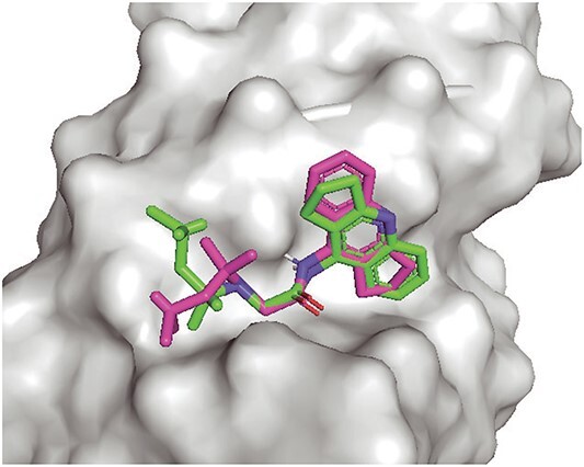
Best pose selected by RmsdXNA (green) and rDock (pink) on PAN triplex RNA.

Screening application validated with MD simulations

The screening power of RmsdXNA and rDock for VS application on MALAT1 was compared by evaluating the MD trajectories of the top ligands selected by each scoring function. RmsdXNA was able to identify about 6 times more stable ligands out of 20 top-scored ligands compared to rDock as shown in Table 3. This finding suggests that RmsdXNA has a higher success rate in identifying potential ligands that binds strongly to the receptor, making it more accurate and reliable for screening. Interestingly, no common top candidate ligands were identified by RmsdXNA and rDock. From the top poses selected by RmsdXNA and rDock as illustrated in Figure 7, it is observed that RmsdXNA tends to give better scores to poses that intercalate between the RNA residues, but no such poses are selected by rDock. This indicates that a change in the score function can result in different outputs. The ability to accurately identify stable ligands is crucial for selecting reliable docking tools and refining computational docking protocols. By improving the efficiency and success rate of VS-related efforts in drug discovery, RmsdXNA can greatly impact the field.

Table 3.

Number of stable ligands from the 20 top-scored ligands selected by RmsdXNA and rDock during the MD simulation of 100 ns. The Chembridge and Life Chemicals screening compound libraries were used for the VS.

Dataset	Number of stable ligands based on MD simulations
	RmsdXNA	rDock
Chembridge	13	2
Life chemicals	12	2

Figure 7.

Poses of the top 20 ligand selected by RmsdXNA and rDock from Chembridge and Life Chemicals screening libraries docked on 4PLX using rDock. Top-scored ligand poses selected by RmsdXNA tend to intercalate between the RNA residues. This is not observed for the top-scored ligands selected by rDock.

Limitations

In this study, RmsdXNA was evaluated and trained on ligand poses generated by local docking, excluding poses with RMSD 10 Åfrom the native pose. This exclusion may limit the functionality of RmsdXNA when the docking pocket is unknown, but it is necessary to reduce noise in the dataset during training and evaluation [63]. RmsdXNA is expected to perform well if docking tools can accurately generate close-to-native ligand poses or address the flexibility issue of the receptor as discussed in Stefaniak and Bujnicki [36]. Furthermore, tools that identify RNA-ligand binding sites [64], can be used in conjunction with RmsdXNA to accurately identify the docking pocket.

The small number of experimentally determined NA–ligand complexes presents a challenge for improving the ML model for NA docking tools. Infrequent feature interaction also hinder the model from learning this information effectively. However, the advantages of easy feature extraction and adaptability to different datasets presented in RmsdXNA simplify the addition of new data points to enhance the accuracy of the model. While RmsdXNA demonstrated overall better results than rDock in validation against PAN triplex MST experiment and MD simulations validation of MALAT1 VS, a wider variety of experimental dataset involving diverse receptors is required to comprehensively evaluate the reliability of the scoring functions for virtual screening and pose identification.

CONCLUSION

RmsdXNA, a ML regression model, was successfully developed and demonstrated to be an effective tool for predicting the RMSD of docked ligand poses in NA complexes. The model incorporates distance-based features that capture atom-atom interactions in NA complexes, including those containing metal ions, modified residues, and peptide ligands. The experiments showed that there is a correlation between the binding affinity and the predicted RMSD of a ligand pose, which can be used for pose identification and screening. RmsdXNA outperformed the other docking tools when evaluated on the testing dataset. It also achieved high prediction accuracy with an average validation of 0.68301 0.02330 and an average PCC of 0.64531 0.36262 and SRCC of 0.58465 0.3519 across the different ligands. The alignment of the scoring ranking with the result of the MST experiments conducted on PAN triplex validated RmsdXNA’s better capability than rDock in distinguishing strong binders from weaker binders. RmsdXNA also has a higher success rate in identifying good ligand candidates for VS, supported by the MD simulations of MALAT1. Overall, this study demonstrated that ML can be utilized to improve the accuracy of molecular docking methodologies in the field of computational drug design.

Author contributions

L.H. was responsible for carrying out all the experimental work, data collection and analysis. Y.G. provided valuable guidance and advice on the methods used in this project, contributing to the overall design and approach. C.K. contributed expertise in data analysis and machine learning modeling, offering insightful advice throughout the analysis phase. All authors read and approved the final manuscript.

Key Points

• The intermolecular atom-atom pairwise distance of docking poses, r, were used to generate and features, which were subsequently used to construct the dataset for training the machine learning model. The model, namely RmsdXNA, is trained on 980 nucleic acid (NA)–ligand complex structure dataset using the XGBoostRegressor algorithm to predict the root-mean-square-deviation (RMSD) of a docked pose.

• Modification of the features used in Wang et al. [41] allows us apply these features from protein–ligand complexes to NA–ligand complex systems in RmsdXNA. The results show successful application of RmsdXNA to various NA–ligand complexes, including different types of NA receptors and ligands.

• The RMSD predicted by RmsdXNA outperforms rDock score in pose identification when evaluated on the testing dataset used in Feng et al. [19].

• RmsdXNA demonstrated better scoring power and pose identification than rDock, using the binding affinities of small molecules on polyadenylated nuclear (PAN) triplex RNA obtained by microscale thermophoresis (MST).

• Molecular dynamics (MD) simulation on MALAT1–ligand complex was performed to validate the binding of the top ligand candidates selected by RmsdXNA and rDock during virtual screening. The results showed that RmsdXNA had a higher success rate in selecting stable ligands by approximately 6 times.

A Appendix

Appendix A. PDB list

The list of PDB structures from NDB used for docking are shown in the list below. The PDB IDs in red are not used in the dataset as the ligands were docked unsuccessfully, where there are fewer than 100 poses out of 400 dock attempts with RMSD 10Å.

100D

101D

102D

108D

109D

110D

121D

127D

128D

129D

130D

131D

144D

151D

152D

154D

159D

166D

173D

182D

185D

193D

195D

198D

1AGL

1AJU

1AKX

1AL9

1AM0

1AMD

1ARJ

1AW4

1BYJ

1C9Z

1CX3

1D10

1D11

1D14

1D17

1D21

1D22

1D30

1D32

1D36

1D37

1D38

1D43

1D44

1D45

1D46

1D48

1D54

1D58

1D63

1D64

1D67

1D85

1D86

1DA0

1DA9

1DB6

1DCR

1DDY

1DJ6

1DL8

1DNE

1DNH

1DNS

1DPL

1DSC

1DSD

1DVL

1EDR

1EEL

1EHT

1EI2

1EI4

1EM0

1ET4

1EVV

1F1T

1F27

1F6C

1FD5

1FDG

1FMN

1FMQ

1FMS

1FN2

1FQ2

1FTD

1FUF

1FYP

1G3X

1G4Q

1G5L

1GJ2

1I0T

1I1P

1I2X

1I2Y

1I3W

1I5V

1I7J

1I9V

1IMR

1IMS

1J7T

1JO2

1JTL

1JUX

1K2L

1K2Z

1K9G

1KCI

1KGK

1KOC

1KOD

1KVH

1L0R

1L1H

1L1V

1LC4

1LEX

1LEY

1LVJ

1M69

1MP7

1MTG

1MWL

1MXK

1N37

1N7A

1N7B

1NAB

1NBK

1NEM

1NJN

1NTA

1NTB

1NZM

1O15

1O9M

1OE5

1OFX

1OLD

1OVF

1P96

1P9X

1PBR

1PIK

1PQQ

1PRP

1PWF

1Q8N

1Q9X

1QCH

1QD3

1QSX

1QV4

1QV8

1R4E

1R68

1RAW

1S2R

1TN2

1TOB

1UNJ

1UNM

1UTS

1UUD

1UUI

1VRO

1VS2

1VTG

1VTH

1VTI

1VTJ

1VZK

1WOE

1X95

1XCS

1XPF

1XVR

1Y0Q

1Y26

1Y27

1Y84

1Y8L

1YKV

1YLS

1YRJ

1YYO

1Z3F

1Z58

1Z5T

1Z8V

1ZJG

1ZPH

1ZPI

1ZZ5

202D

206D

209D

210D

211D

215D

216D

217D

224D

227D

231D

234D

236D

245D

248D

258D

261D

263D

264D

267D

268D

269D

276D

278D

282D

288D

289D

292D

293D

296D

298D

2A04

2A5R

2ADW

2ARG

2AU4

2B0K

2B2B

2B3E

2B57

2BE0

2BEE

2CKY

2D47

2D55

2DA8

2DBE

2DCG

2DND

2DYW

2EES

2EET

2EEU

2EEV

2EEW

2ELG

2ESI

2ESJ

2ET0

2ET3

2ET4

2ET8

2EZF

2EZG

2F4S

2F4T

2F4U

2F8W

2FCX

2FCY

2FCZ

2FD0

2G5K

2G9C

2GB9

2GCV

2GDI

2GIS

2GJB

2GVR

2GWA

2GYX

2H0W

2H0Z

2HO6

2HO7

2HOJ

2HOM

2HOO

2HOP

2HRI

2I2I

2I5A

2IE1

2JUK

2JWQ

2KD4

2KGP

2KMJ

2KTZ

2KU0

2KX8

2KXM

2L1V

2L7V

2L8H

2L94

2LLJ

2LWH

2LWK

2M4Q

2MB3

2MCC

2MCO

2MG8

2MGN

2MIY

2MS6

2MXS

2N0J

2N6C

2N96

2NEO

2NLM

2NZ4

2O1I

2O3V

2O3W

2O3X

2O3Y

2O43

2O45

2OE5

2OE8

2OEY

2OYQ

2PIK

2PL8

2PWT

2QWY

2R2U

2RF3

2TOB

2TRA

2XNW

2XNZ

2XO1

2YDH

2YGH

2YIE

2Z74

2Z75

302D

303D

304D

305D

306D

308D

311D

316D

319D

320D

321D

323D

324D

326D

328D

336D

352D

355D

358D

360D

367D

375D

385D

386D

3AJK

3AJL

3B4A

3B4B

3B4C

3BNQ

3BNR

3C3Z

3C44

3C5D

3C7R

3CCO

3CDM

3CE5

3D0U

3D2G

3D2V

3D2X

3DIG

3DIL

3DIM

3DIO

3DIQ

3DIR

3DIX

3DIY

3DIZ

3DJ0

3DJ2

3DS7

3DVV

3E5C

3E5E

3E5F

3EGZ

3EM2

3EQW

3ERU

3ES0

3ET8

3EUI

3EUM

3EY0

3EY2

3EY3

3F2Q

3F2T

3F2W

3F2X

3F2Y

3F30

3F4E

3F4G

3F4H

3FO4

3FO6

3FT6

3FU2

3FWO

3FX8

3G4M

3G8T

3G96

3G9C

3GAO

3GCA

3GER

3GES

3GJH

3GJJ

3GOG

3GOT

3GSJ

3GSK

3GX2

3GX3

3GX5

3GX6

3GX7

3I1D

3I5L

3IQN

3IQR

3IRW

3JQ4

3K1V

3L3C

3LA5

3MIJ

3MUM

3MUR

3MUT

3MUV

3MXH

3N4O

3NP6

3NPN

3NPQ

3NX5

3NYP

3NZ7

3OIE

3OMJ

3OZ3

3OZ5

3Q3Z

3Q50

3QCR

3QF8

3QRN

3QSC

3QSF

3RKF

3S4P

3SC8

3SD3

3SKI

3SKL

3SKR

3SKT

3SKW

3SKZ

3SLM

3SLQ

3SUH

3SUX

3T5E

3TD1

3TZR

3U05

3U08

3U0U

3U38

3U4M

3UVF

3UXW

3UYB

3UYH

3V7E

3WRU

403D

407D

410D

428D

432D

442D

443D

447D

448D

449D

452D

453D

454D

459D

465D

473D

474D

482D

4AGZ

4AH0

4AH1

4AOB

4B5R

4BZT

4BZU

4BZV

4D9X

4D9Y

4DA3

4DAQ

4E1U

4E7Y

4E8K

4E8M

4E8N

4E8P

4E8Q

4E8R

4E8S

4E8T

4E8V

4E8X

4E95

4ERJ

4ERL

4F8U

4F8V

4FAQ

4FAR

4FAU

4FAW

4FAX

4FB0

4FE5

4FEJ

4FEL

4FEN

4FEO

4FEP

4FRG

4FRN

4FXM

4G0F

4GPW

4GPX

4GPY

4GQJ

4GXY

4HIF

4HQI

4I9V

4IJ0

4ITD

4JD8

4JF2

4JIY

4K31

4K32

4KQY

4KZD

4L5K

4L81

4LTF

4LTG

4LTH

4LTI

4LTJ

4LTK

4LTL

4LVV

4LVW

4LVX

4LVY

4LVZ

4LW0

4LX5

4LX6

4M3I

4M3V

4MJ9

4MS5

4NFO

4NYA

4NYB

4NYC

4NYD

4NYG

4O5W

4O5X

4OQU

4P1D

4P20

4P3S

4P5J

4P95

4PDQ

4Q9Q

4Q9R

4QIO

4QK8

4QK9

4QKA

4QLM

4QLN

4QVI

4R4A

4R8J

4RE7

4RZD

4TS0

4TS2

4TZX

4TZY

4U8A

4U8B

4U8C

4W90

4W92

4X18

4X1A

4XNR

4XW7

4XWF

4Y1I

4Y1J

4Y1M

4YAZ

4YB0

4YMC

4ZC7

4ZNP

5BJO

5BJP

5BTP

5C45

5C7U

5C7W

5CCW

5CDB

5D5L

5DAM

5DE5

5DHB

5ET2

5FK1

5FK4

5FK5

5FK6

5FKE

5FKF

5FKG

5FKH

5HBW

5HIX

5IP8

5IU5

5IWJ

5JEU

5JEV

5JLW

5KPY

5KRG

5KVJ

5KX9

5L00

5LFS

5LFW

5LFX

5LIG

5LIT

5LWJ

5MVB

5NPM

5O62

5O69

5OB3

5SWE

5T4W

5T83

5TPY

5UED

5UEE

5UX3

5UZA

5V0H

5V0O

5V1L

5V3F

5V9Z

5VCF

5VCI

5VJ9

5VJB

5W77

5XI1

5XJZ

5XZ1

5Z1H

5Z1I

5Z71

5Z80

5Z8F

5ZEI

5ZEJ

6AST

6AZ4

6BFB

6BNA

6BST

6C63

6C64

6C65

6C8E

6C8K

6C8L

6C8M

6C8O

6CB3

6CC1

6CC3

6CCW

6CHR

6CIL

6CK4

6CK5

6D8A

6DB8

6DLQ

6DLR

6DLS

6DLT

6DMC

6DMD

6DME

6DN1

6DN2

6DN3

6DY5

6E1S

6E1U

6E1V

6E1W

6E84

6E8T

6E8U

6FC9

6FZ0

6G7Z

6G8S

6GIM

6GYV

6GZK

6GZR

6HAG

6HBT

6HBX

6HC5

6HMO

6HWG

6IJV

6IJW

6J0H

6J2W

6JBF

6JBG

6JJ0

6JJH

6JJI

6JWD

6JWE

6K3Y

6KFI

6KFJ

6KFL

6KN4

6KXZ

6LNZ

6M4T

6M5B

6M5J

6N5K

6N5N

6N5O

6N5P

6N5Q

6N5S

6N5T

6O2L

6OD9

6P2H

6P45

6PNK

6PQ7

6Q57

6QIV

6QN3

6R6D

6RNL

6RSO

6RTI

6S15

6S7D

6SX3

6T3K

6T3N

6T3R

6T3S

6TB7

6TF0

6TF1

6TF2

6TF3

6TFE

6TFF

6TFG

6TFH

6U6J

6U7Y

6U7Z

6U89

6U8F

6U8U

6UBU

6UC7

6UC8

6UC9

6UP0

6V0L

6V9D

6VA2

6VA3

6VA4

6VMY

6VUI

6VWT

6VWV

6WTL

6WTR

6WZR

6WZS

6XB7

6XCL

6XKN

6XKO

6XRQ

6XT7

6YL5

6YLB

6YMI

6YMJ

6YMK

6YML

6YMM

7A3Y

7ATG

7CPS

7CSK

7D12

7D5E

7D7W

7D7X

7D7Y

7D7Z

7D81

7D82

7DFY

7DJU

7DJV

7DJW

7DWH

7E9E

7E9I

7EAF

7EDL

7EDM

7EDT

7EL7

7ELP

7ELQ

7ELR

7ELS

7EOG

7EOH

7EOI

7EOJ

7EOK

7EOL

7EOM

7EON

7EOO

7EOP

7FHI

7FJ0

7JNH

7KBW

7KBX

7KLP

7KU4

7KUK

7KUL

7KUM

7KUN

7KUO

7KUP

7KVT

7KVU

7KVV

7KWK

7L0Z

7LNE

7LNF

7LNG

7MSV

7N7D

7N7E

7OA3

7OAV

7OAW

7OAX

7OTB

7PNG

7Q7X

7Q7Y

7Q7Z

7Q80

7Q81

7Q82

7RWR

7SZU

7TD7

7TDA

7TDB

7TDC

7TZR

7TZS

7TZT

7TZU

7V9E

7W9N

7WGW

7X2Z

7X3A

7XLV

1AO1

1LEJ

2RSK

2RU7

4GMA

5DE8

5ODF

5ODM

5OE1

6E8S

6GZ7

6I4N

6LEW

6RIO

7FGT

7RIL

Appendix B. Data refinement for data preparation

All NA molecules selected using bymolecule entity expansion and protein chains with masses greater than 1500 atomic units (au) were labeled as receptors. The protein receptor was removed during docking.

The following data refinements are performed for data preparation:

• The remaining molecules that are not labeled as receptors, excluding solvent molecules or molecules with fewer than 6 heavy atoms, are labeled as ligands.

• A bond is added between an unbonded residue and the NA receptor if the distance between the atoms is 1.65 Å to fix the missing bond in the structure, and these residues are treated as the receptors.

• Ligands with a mass larger than 1500 au were removed. This process filters away large ligands or proteins that are highly flexible and may act as noise for the model [63].

• Ligands that were closer than (radius of gyration of ligand + 10 Å) from a protein receptor removed to exclude ligands with conformations that may be affected by nearby protein receptors.

• In cases where the NA-ligand complexes contained multiple ligands, only ligands more than 4.0 Å from each other were used for docking, while the other ligands were removed from the dataset. This is because ligands that are nearby may influence each others’ native pose. The absence of nearby ligands when performing docking may undermine the accuracy of the model in predicting the RMSD of the docked poses. Additionally, identical ligands in close proximity may result in incorrect reference pose being used for predicting the RMSD of the docked pose if the docking pockets are nearby.

• For structures with alternative conformations, the first variant is used for receptor atoms, while complexes with alternative conformations in the ligand are removed. This prevents the problem of having multiple references of the ligand’s native poses when measuring the RMSD of the docked poses.

• Only the first model is used for structures solved using nuclear magnetic resonance.

• Complexes without any valid ligand molecules were excluded from the experiment.

List of residue names of molecules that are labeled as solvent and not used as ligand for docking: 13D, 1PE, ACT, AGU, ARF, BA, BCT, BME, BR, CL, CON, CPT, DMS, EDO, EOH, FMT, GAI, GLY, GOL, GZ6, IPA, IRI, MGX, MOH, NCO, NRU, OHX, PDO, PGE, PO4, PTN, RHD, RUH, SE4, SEY, SO4, TEA, TMO, URE,

Appendix C. NA and ligand atom groups

Table A1.

Atom group of the receptor atoms in ’OTH’ residue group based on its SYBYL atom type. The atoms are grouped according to their element, while the halogens are grouped into a ’Hal’ group. For modified residues containing ’O.co2’ and ’P.3’ atoms, since these atoms appear in the backbone and ribose structure (N), ’N’ residue type is assigned to the receptor atoms containing ’O.co2’ and ’P.3’.

Atom Group	SYBYL atom type
O	O.2, O.3
C	C.2, C.3
N	N.2, N.3, N.4, N.pl3
Hal	Br, Cl, F, I

Table A1 shows the grouping of the receptor atoms in 'OTH' residue group. For ligand atom type, C.cat (carbocation in a guadinium group) and C.2 (carbon sp2) SYBYL atom types are grouped together to form C2 atom group. C.cat in the ligand only appeared in 6 PDB structures, therefore binning the features formed by C.cat ligand can reduce the sparsity of the dataset and improve the result.

Table A2.

Atom types considered in feature generation. The SYBYL atom types of the canonical residues is based on the atom name of the atom as shown in Appendix E. Italicized atom types are grouped by the methods above shown in Appendix C. 24 ligand atom types for ligand and 26 NA atom types (unique combinations of the atom types that appear in each residue type) were used, resulting in 624 pair of interactions.

Receptor		Ligand
Residue	Atom type	Atom type
A	N.ar, C.ar, N.pl3	C2, C.1, C.3, C.ar, Br, Cl, F, I, N.1, N.2, N.3, N.4, N.am, N.ar, N.pl3 O.2, O.3, O.co2, S.2, S.3, S.O2, P.3, Se, Metal
G	N.ar, C.ar, N.pl3, O.2
C	N.ar, C.ar, N.pl3, O.2
U/T	N.ar, C.ar, O.2, C.3
N	P.3, C.3, O.3, O.co2
OTH	O, C, N, Hal, Se, S.3
Metal	Metal

After grouping the receptor and ligand atom types as mentioned above, the atom type representations are shown in Table A2. Columns with all 0 values were removed from the dataset and used to train the model.

Appendix D. Residue type generalization

The generalization of modified NA residues into the unmodified NA residues based on structural similarity. For each modified residue structure, the atoms that are similar to the ”parent” nucleotide in terms of its position are represented in sticks (thicker) and the atoms are represented by SYBYL atom type for feature generation. On the other hand, the other modified atoms are represented in lines (thinner) and the atoms are represented by their element for feature generation. Visualization of the structures was performed using PyMol.

For new residues that are not shown in this section, similar residue generalization and atom representation methods can be applied for feature generation.

Appendix E. Atom name and SYBYL atom type of residues A, C, G, U/T

of receptor atom that are in the canonical nucleobase position is the classified RNA’s nucleobases group; of receptor atom in the ribose and phosphate backbone is ’N’; of the metal atoms in the receptor is ’Metal’, while for the other atoms is ’OTH’. is represented by the SYBYL atom type based on its position as shown in Figure A1 and Table A3.

Figure A1.

The atom names of residues A, G, C, U/T.

Table A3.

The SYBYL atom type representation of the atoms in nucleobases A, C, G, U/T and the backbone (N) based on the atom’s position as shown in Figure A1

Residue	SYBYL atom type	Atom name
A	N.ar	N1, N3, N7, N9
	C.ar	C2, C4, C5, C6, C8
	N.pl3	N6
G	N.ar	N1, N3, N7, N9
	C.ar	C2, C4, C5, C6, C8
	O.2	O6
	N.pl3	N2
C	N.ar	N1, N3
	C.ar	C2, C4, C5, C6
	N.pl3	N4
	O.2	O2
U/T	N.ar	N1, N3
	C.ar	C2, C4, C5, C6
	O.2	O2, O4
	C.3	C7
N	P.3	P
	C.3	C5’, C1’, C2’, C3’, C4’
	O.3	O5’, O3’, O2’, O4’
	O.co2	OP1, OP2

Appendix F. Hyperparameter values for the best performing model

max_depth: 13, n_estimators: 900, min_child_weight: 5, learning_rate: 0.02, subsample: 0.3, colsample_bytree: 0.4, reg_alpha: 1, reg_lambda: 1, gamma:1, rate_drop: 0.3,

Appendix G. Best result of other ML models

Table A4.

The best obtained for different algorithms. All algorithms perform worse than XGBoost, which has a = 0.68301.

Algorithm	Best
Multilayer Perceptron	0.43258
AdaBoost	0.41016
Random Forest	0.65553
Support Vector Regression	0.57900

Appendix H. MD simulation protocol

To prepare for the MD simulations, the force fields of the receptor and ligands were generated using AMBER [65]. Then, the AMBER topologies are converted to GROMACS [66] format using ANTECHAMBER [67] and ParmEd software [68] (https://github.com/ParmEd/ParmEd). MD simulations of the MALAT1-ligand complex in water with 0.15 M sodium chloride ions at 300 K and the TIP3P water model [69] were performed using GROMACS simulation software to generate a 100 ns trajectory.

Appendix I. Structure of screening compounds

Figure A2.

The atom names of residues A, G, C, U/T.

Appendix J. Ablation studies results - cutoff distance

Table A5.

Average validating of actual vs. predicted ligand pose RMSD values, , trained on datasets generated using cutoff distance of 4 to 10 Å for feature generation. The value and its standard deviation (std) is calculated from the validating obtained from each fold in the 5-fold cross-validation training. nfeatures shows the number of features in the dataset, and the % 0 in dataset measures the sparsity of the dataset.

cutoff distance,	nfeature	% 0 in dataset (%)		std
4	1040	92.1	0.64660	0.02483
5	1062	89.2	0.66621	0.02018
6	1072	86.9	0.67458	0.01980
7	1082	84.7	0.67742	0.01882
8	1088	83.1	0.68301	0.02330
9	1092	82.0	0.67929	0.01941
10	1098	81.3	0.68176	0.02061

Appendix K. Ablation studies results - feature combinations

Table A6.

Average validating of actual vs. predicted ligand pose RMSD values, , trained using datasets generated using combinations of rDock, , and features. rDock feature represent the components generated from rDock scoring function, while the , and features represents the features used to describe the intermolecular force field energy as shown in Section 2.3.

Feature	nfeature		std
rDock	30	0.48328	0.03950
rDock +	559	0.66988	0.02106
rDock +	559	0.6737	0.02028
rDock +	559	0.66803	0.0210
rDock + + (default)	1088	0.68301	0.02330
rDock + +	1088	0.67798	0.01998
rDock + +	1088	0.67601	0.01964
rDock + + +	1619	0.67910	0.01763
+	1060	0.65344	0.02865
+ +	1591	0.65241	0.02956

Appendix L. Ablation studies results - feature binning

Table A7.

Average validating of actual vs. predicted ligand pose RMSD values, , for the best models from datasets generated by different atom representations. The receptor and ligand atoms are represented in either default (Appendix C), element, or SYBYL MOL2 format. The highest average validating of 0.68301 is obtained for the default dataset.

Modification name	nfeature		std	Atom representation
				Receptor	Ligand
atomgroup (default)	1088	0.68301	0.02330	Default	Default
ligandelem	516	0.67128	0.02350	Default	Element
ligandmol2	1126	0.68173	0.0206	Default	SYBYL MOL2
recelem	850	0.67447	0.02168	Element	Default
recmol2	1174	0.68209	0.0184	SYBYL MOL2	Default
ligandrecelem	408	0.66726	0.02244	Element	Element
ligandrecmol2	1256	0.67945	0.01654	SYBYL MOL2	SYBYL MOL2

Appendix M. Ligand analysis

Table A8.

List of ligands with similar structures and relatively high PCC between the actual RMSD of the poses and RmsdXNA predicted RMSD.

(a) List of PDB IDs with structure containing ruthenium polypyridyl-like complex ligands and its PCC values.		(b) List of PDB IDs with structure containing hypoxanthine-like ligands and its PCC values
PDB ID	PCC of ligand	PDB ID	PCC of ligand
4R8J	0.99890	4FEN	0.99755
4LTF	0.99748	4FEL	0.99568
5LFW	0.99559	7V9E	0.99272
4LTJ	0.99521	7Q7Y	0.99260
3UYB	0.99455	2EEU	0.99238
4E8S	0.99202	4FEJ	0.99174
4E1U	0.98948	2EET	0.98871
5LFX	0.98790	1Y27	0.98822
4M3V	0.98708	7Q80	0.98757
4JD8	0.98595	4FE5	0.98755

Appendix N. Testing data list from NLDock

The list of PDB IDs from Feng et al. [19] that are used for the testing data are shown in the list below. The PDB IDs in red are not used in the testing dataset and are missing from the dataset, due to the filter criteria when selecting the PDB structures. Table A9 shows the number of NA-ligand structures in the test dataset and the number of ligands that are used for the evaluation of RmsdXNA.

1AJU	1AKX	1AM0	1ARJ	1BYJ	1DB6	1EHT	1EI2	1F1T	1F27	1FMN
1FYP	1I9V	1J7T	1KOC	1KOD	1LC4	1LVJ	1MWL	1NBK	1NEM	1NTA
1NTB	1NZM	1O15	1O9M	1P96	1PBR	1Q8N	1QD3	1QV4	1QV8	1R4E
1TOB	1UTS	1UUD	1UUI	1XPF	1Y26	1Y27	1YKV	1YRJ	1ZZ5	2AU4
2B57	2BE0	2BEE	2D55	2ESI	2ESJ	2ET3	2ET4	2ET8	2F4S	2F4T
2F4U	2FCX	2FCY	2FCZ	2FD0	2G9C	2GDI	2GIS	2JUK	2JWQ	2KGP
2KTZ	2KU0	2KX8	2L94	2MB3	2O3V	2O3W	2O3X	2OE5	2OE8	2PWT
2TOB	2XNW	2XNZ	2XO1	2YDH	2YGH	2Z74	2Z75	316D	3C44	3D2X
3DIL	3DS7	3DVV	3E5C	3F2Q	3FO4	3FO6	3FU2	3G4M	3GAO	3GER
3GES	3GOG	3GOT	3GX2	3GX3	3GX5	3GX7	3LA5	3MUM	3MUR	3MXH
3NPN	3NPQ	3Q3Z	3Q50	3S4P	3SD3	3SLM	3SUX	407D	4AOB	4ERJ
4FE5	4JF2	4KQY	4LVV
1CVX	1CVY	1F4S	1FJG	1G5K	1HNW	1NYI	1U8D	1XBP	2G5Q	2LOA
2OGN	2XO0	3OWZ	408D

Table A9.

The full number of PDB structures in the NA-ligand test dataset and the number of ligands that were used in our dataset.

Dataset	No. of structures in dataset	No. of structures used
Yan	77	69
Ruiz	56	53
Chen	56	54
Philips	42	37

Appendix O. Ranking of compounds based on their binding affinity and scores

Table A10.

Binding affinities of hit compounds by Swain et al. [42] and the RmsdXNA and rDock scores of the best pose selected by each scoring method. The compounds are also ranked based on their binding affinity and scores.

Compound	Binding Affinity	Binding Affinity rank	RmsdXNA score	RmsdXNA rank	rDock score	rDock rank
8	700 M	5	5.974	2	-18.572	3
13	305 M	4	5.387	1	-18.678	2
15	27 M	1	6.415	4	-18.153	5
18	3.2 mM	7	6.865	6	-18.336	4
19	800 M	6	6.988	7	-13.614	7
20	128 M	2	6.319	3	-19.418	1
25	209 M	3	6.836	5	-16.083	6

Table A11.

The RmsdXNA and rDock scores and score ranking of the best pose selected by each scoring method for Compound 15 and its modification counterparts.

Compound	RmsdXNA score	RmsdXNA rank	rDock score	rDock rank
15	6.415	2	-18.153	4
15-A1	6.621	3	-18.841	3
15-A2	6.616	4	-25.707	1
15-A3	6.247	1	-21.201	2

FUNDING

This research was supported by Singapore Ministry of Education (MOE) Tier 1 grants RG27/21 and RG97/22. Computations were mainly performed using the resources of the National Supercomputing Centre, Singapore (https://www.nscc.sg) and the HADLEY high-performance computing cluster of SCELSE. SCELSE is funded by Singapore’s National Research Foundation, the Ministry of Education, NTU, and the National University of Singapore (NUS), and is hosted by NTU in partnership with NUS.

DATA AVAILABILITY

The data underlying this article are available in the article and in its online supplementary material.

References

- 1. Hopkins AL, Groom CR. The druggable genome. Nat Rev Drug Discov 2002; 1(9): 727–30. [DOI] [PubMed] [Google Scholar]
- 2. Gurevich EV, Gurevich VV. Therapeutic potential of small molecules and engineered proteins. Arrestins-Pharmacol Therapeutic Potential 2014; 219:1–12. [DOI] [PMC free article] [PubMed] [Google Scholar]
- 3. Kulkarni JA, Witzigmann D, Thomson SB, et al. The current landscape of nucleic acid therapeutics. Nat Nanotechnol 2021; 16(6): 630–43. [DOI] [PubMed] [Google Scholar]
- 4. Morris KV, Mattick JS. The rise of regulatory rna. Nat Rev Genet 2014; 15(6): 423–37. [DOI] [PMC free article] [PubMed] [Google Scholar]
-
5.
Lawrence CW. Cellular roles of DNA polymerase
and Rev1 protein. DNA Repair 2002; 1(6): 425–35.
[DOI] [PubMed] [Google Scholar]
[DOI] [PubMed] [Google Scholar] - 6. Chu G. Cellular responses to cisplatin. The roles of DNA-binding proteins and dna repair. J Biol Chem 1994; 269(2): 787–90. [PubMed] [Google Scholar]
- 7. Wild EJ, Tabrizi SJ. Therapies targeting dna and rna in huntington’s disease. Lancet Neurol 2017; 16(10): 837–47. [DOI] [PMC free article] [PubMed] [Google Scholar]
- 8. Monroig P d C, Chen L, Zhang S, Calin GA. Small molecule compounds targeting miRNAs for cancer therapy. Adv Drug Deliv Rev 2015; 81:104–16. [DOI] [PMC free article] [PubMed] [Google Scholar]
- 9. Gurova K. New hopes from old drugs: revisiting dna-binding small molecules as anticancer agents. Future Oncol 2009; 5(10): 1685–704. [DOI] [PMC free article] [PubMed] [Google Scholar]
- 10. Tili E, Michaille J-J, Croce CM. Micro rna s play a central role in molecular dysfunctions linking inflammation with cancer. Immunol Rev 2013; 253(1): 167–84. [DOI] [PubMed] [Google Scholar]
- 11. Shemiakova T, Ivanova E, Grechko AV, et al. Mitochondrial dysfunction and dna damage in the context of pathogenesis of atherosclerosis. Biomedicine 2020;8. [DOI] [PMC free article] [PubMed] [Google Scholar]
- 12. Brown RF, Andrews CT, Elcock AH. Stacking free energies of all dna and RNA nucleoside pairs and dinucleoside-monophosphates computed using recently revised amber parameters and compared with experiment. J Chemical Theory Comput 2015; 11:2315–28. [DOI] [PMC free article] [PubMed] [Google Scholar]
- 13. Chauvot I, Beauchene de SJ, Vries de, and Martin Zacharias. Binding site identification and flexible docking of single stranded rna to proteins using a fragment-based approach. PLoS Comput Biol 2016; 12(1): e1004697. [DOI] [PMC free article] [PubMed] [Google Scholar]
- 14. Ma H, Jia X, Zhang K, Zhaoming S. Cryo-em advances in RNA structure determination. Signal Transduct Target Ther 2022; 7(1): 58. [DOI] [PMC free article] [PubMed] [Google Scholar]
- 15. Velagapudi SP, Luo Y, Tran T, et al. Defining RNA–small molecule affinity landscapes enables design of a small molecule inhibitor of an oncogenic noncoding RNA. ACS Central Science 2017; 3(3): 205–16. [DOI] [PMC free article] [PubMed] [Google Scholar]
- 16. Daldrop P, Brenk R. Structure-based virtual screening for the identification of RNA-binding ligands. Therapeutic Appl Ribozymes Riboswitches: Methods Protocols 2014; 1103:127–39. [DOI] [PubMed] [Google Scholar]
- 17. Meng X-Y, Zhang H-X, Mezei M, Cui M. Molecular docking: a powerful approach for structure-based drug discovery. Curr Comput Aided Drug Des 2011; 7(2): 146–57. [DOI] [PMC free article] [PubMed] [Google Scholar]
- 18. Ruiz-Carmona S, Alvarez-Garcia D, Nicolas Foloppe A, et al. Rdock: a fast, versatile and open source program for docking ligands to proteins and nucleic acids. PLoS Comput Biol 2014; 10(4): e1003571. [DOI] [PMC free article] [PubMed] [Google Scholar]
- 19. Feng Y, Zhang K, Qilong W, Huang S-Y. Nldock: a fast nucleic acid–ligand docking algorithm for modeling RNA/DNA–ligand complexes. J Chem Inf Model 2021; 61(9): 4771–82. [DOI] [PubMed] [Google Scholar]
- 20. Sun L-Z, Jiang Y, Zhou Y, Chen S-J. Rldock: a new method for predicting RNA–ligand interactions. J Chemical Theory Comput 2020; 16(11): 7173–83. [DOI] [PMC free article] [PubMed] [Google Scholar]
- 21. Morris GM, Lim-Wilby M. Molecular docking. Mol Modeling Proteins 2008; 443:365–82. [DOI] [PubMed] [Google Scholar]
- 22. Kitchen DB, Decornez H, Furr JR, Bajorath J. Docking and scoring in virtual screening for drug discovery: methods and applications. Nat Rev Drug Discov 2004; 3(11): 935–49. [DOI] [PubMed] [Google Scholar]
- 23. Wang M, Yuanyuan Y, Liang C, et al. Recent advances in developing small molecules targeting nucleic acid. Int J Mol Sci 2016; 17(6): 779. [DOI] [PMC free article] [PubMed] [Google Scholar]
- 24. Lim S, Yijingxiu L, Cho CY, et al. A review on compound-protein interaction prediction methods: data, format, representation and model. Comput Struct Biotechnol J 2021; 19:1541–56. [DOI] [PMC free article] [PubMed] [Google Scholar]
- 25. Saikia S, Bordoloi M. Molecular docking: challenges, advances and its use in drug discovery perspective. Curr Drug Targets 2019; 20(5): 501–21. [DOI] [PubMed] [Google Scholar]
- 26. Genheden S, Ryde U. The mm/pbsa and mm/gbsa methods to estimate ligand-binding affinities. Expert Opin Drug Discovery 2015; 10(5): 449–61. [DOI] [PMC free article] [PubMed] [Google Scholar]
- 27. Kuhn M, Firth-Clark S, Tosco P, et al. Assessment of binding affinity via alchemical free-energy calculations. J Chem Inf Model 2020; 60:3120–30. [DOI] [PubMed] [Google Scholar]
- 28. Melville JL, Burke EK, Hirst JD. Machine learning in virtual screening. Comb Chem High Throughput Screen 2009; 12(4): 332–43. [DOI] [PubMed] [Google Scholar]
- 29. Masters MR, Mahmoud AH, Wei Y, Lill MA. Deep learning model for efficient protein–ligand docking with implicit side-chain flexibility. J Chem Inf Model 2023; 63(6): 1695–707. [DOI] [PubMed] [Google Scholar]
- 30. Crampon K, Giorkallos A, Deldossi M, et al. Machine-learning methods for ligand–protein molecular docking. Drug Discov Today 2022; 27(1): 151–64. [DOI] [PubMed] [Google Scholar]
- 31. Shen C, Ding J, Wang Z, et al. From machine learning to deep learning: advances in scoring functions for protein–ligand docking. Wiley Interdiscipl Rev: Comput Mol Sci 2020; 10(1): e1429. [Google Scholar]
- 32. Feng Y, Huang S-Y. Itscore-nl: an iterative knowledge-based scoring function for nucleic acid–ligand interactions. J Chem Inf Model 2020; 60(12): 6698–708. [DOI] [PubMed] [Google Scholar]
- 33. Feng Y, Yan Y, He J, et al. Docking and scoring for nucleic acid–ligand interactions: principles and current status. Drug Discov Today 2022; 27(3): 838–47. [DOI] [PubMed] [Google Scholar]
- 34. Zhou Y, Jiang Y, Chen S-J. Rna–ligand molecular docking: advances and challenges. Wiley Interdiscipl Rev: Comput Mol Sci 2022; 12(3): e1571. [DOI] [PMC free article] [PubMed] [Google Scholar]
- 35. Chhabra S, Xie J, Frank AT. Rnaposers: machine learning classifiers for ribonucleic acid–ligand poses. J Phys Chem B 2020; 124(22): 4436–45. [DOI] [PubMed] [Google Scholar]
- 36. Stefaniak F, Bujnicki JM. Annapurna: a scoring function for predicting rna-small molecule binding poses. PLoS Comput Biol 2021; 17(2): e1008309. [DOI] [PMC free article] [PubMed] [Google Scholar]
- 37. Duffy K, Arangundy-Franklin S, Holliger P. Modified nucleic acids: replication, evolution, and next-generation therapeutics. BMC Biol 2020; 18(1): 1–14. [DOI] [PMC free article] [PubMed] [Google Scholar]
- 38. Peselis A, Serganov A. Structural insights into ligand binding and gene expression control by an adenosylcobalamin riboswitch. Nat Struct Mol Biol 2012; 19(11): 1182–4. [DOI] [PubMed] [Google Scholar]
- 39. Cuesta-Seijo JA, Sheldrick GM. Structures of complexes between echinomycin and duplex dna. Acta Crystallogr D Biol Crystallogr 2005; 61(4): 442–8. [DOI] [PubMed] [Google Scholar]
- 40. Chen X, Ramakrishnan B, Sundaralingam M. Crystal structures of b-form dna-rna chimers complexed with distamycin. Nat Struct Biol 1995; 2(9): 733–5. [DOI] [PubMed] [Google Scholar]
- 41. Wang Z, Zheng L, Wang S, et al. A fully differentiable ligand pose optimization framework guided by deep learning and a traditional scoring function. Brief Bioinform 2023a; 24(1):bbac520. [DOI] [PubMed] [Google Scholar]
- 42. Swain M, Ageeli AA, Kasprzak WK, et al. Dynamic bulge nucleotides in the kshv pan ene triple helix provide a unique binding platform for small molecule ligands. Nucleic Acids Res 2021; 49(22): 13179–93. [DOI] [PMC free article] [PubMed] [Google Scholar]
- 43. Berman HM, Olson WK, Beveridge DL, et al. The nucleic acid database. A comprehensive relational database of three-dimensional structures of nucleic acids. Biophys J 1992; 63:751–9. [DOI] [PMC free article] [PubMed] [Google Scholar]
- 44. Narayanan BC, Westbrook J, Ghosh S, et al. The nucleic acid database: new features and capabilities. Nucleic Acids Res 2014; 42(D1): D114–22. [DOI] [PMC free article] [PubMed] [Google Scholar]
- 45. The pymol molecular graphics system, version 2.0 schrödinger, llc.
- 46. Yan Z, Wang J. Spa-ln: a scoring function of ligand–nucleic acid interactions via optimizing both specificity and affinity. Nucleic Acids Res 2017; 45(12): e110–0. [DOI] [PMC free article] [PubMed] [Google Scholar]
- 47. Morris GM, Goodsell DS, Huey R, et al. Autodock. Automated Docking of Flexible Ligands to Receptor-User Guide, 2001.
- 48. Meli R, Biggin PC. Spyrmsd: symmetry-corrected rmsd calculations in python. J Chem 2020; 12(1): 49. [DOI] [PMC free article] [PubMed] [Google Scholar]
- 49. Zheng L, Fan J, Yuguang M. Onionnet: a multiple-layer intermolecular-contact-based convolutional neural network for protein–ligand binding affinity prediction. ACS Omega 2019; 4(14): 15956–65. [DOI] [PMC free article] [PubMed] [Google Scholar]
- 50. Wang Z, Zheng L, Liu Y, et al. Onionnet-2: a convolutional neural network model for predicting protein-ligand binding affinity based on residue-atom contacting shells. Front Chem 2021; 9:753002. [DOI] [PMC free article] [PubMed] [Google Scholar]
- 51. Taminau J, Thijs G, De Winter. Pharao: pharmacophore alignment and optimization. J Mol Graph Model 2008; 27(2): 161–9. [DOI] [PubMed] [Google Scholar]
- 52. Boniecki MJ, Lach G, Dawson WK, et al. Simrna: a coarse-grained method for rna folding simulations and 3d structure prediction. Nucleic Acids Res 2016; 44(7): e63–3. [DOI] [PMC free article] [PubMed] [Google Scholar]
- 53. Minyi S, Du Qifan Yang, Feng G, et al. Comparative assessment of scoring functions: the casf-2016 update. J Chem Inf Model 2018; 59(2): 895–913. [DOI] [PubMed] [Google Scholar]
- 54. Hansson T, Oostenbrink C, Gunsteren van. Molecular dynamics simulations. Curr Opin Struct Biol 2002; 12(2): 190–6. [DOI] [PubMed] [Google Scholar]
- 55. Alnajjar R, Mostafa A, Kandeil A, Al-Karmalawy AA. Molecular docking, molecular dynamics, and in vitro studies reveal the potential of angiotensin ii receptor blockers to inhibit the covid-19 main protease. Heliyon 2020; 6(12): e05641. [DOI] [PMC free article] [PubMed] [Google Scholar]
- 56. Brown JA, Kinzig CG, DeGregorio SJ, Steitz JA. Methyltransferase-like protein 16 binds the 3-terminal triple helix of malat1 long noncoding rna. Proc Natl Acad Sci 2016; 113(49): 14013–8. [DOI] [PMC free article] [PubMed] [Google Scholar]
- 57. Brown JA, Bulkley D, Wang J, et al. Structural insights into the stabilization of malat1 noncoding rna by a bipartite triple helix. Nat Struct Mol Biol 2014; 21:633–40. [DOI] [PMC free article] [PubMed] [Google Scholar]
- 58. Okimoto N, Futatsugi N, Fuji H, et al. High-performance drug discovery: computational screening by combining docking and molecular dynamics simulations. PLoS Comput Biol 2009; 5(10): e1000528. [DOI] [PMC free article] [PubMed] [Google Scholar]
- 59. Szulc NA, Mackiewicz Z, Bujnicki JM, Stefaniak F. Fingernat—a novel tool for high-throughput analysis of nucleic acid-ligand interactions. PLoS Comput Biol 2022; 18(6): e1009783. [DOI] [PMC free article] [PubMed] [Google Scholar]
- 60. Padroni G, Patwardhan NN, Schapira M, Hargrove AE. Systematic analysis of the interactions driving small molecule–rna recognition. RSC Medicinal Chemistry 2020; 11(7): 802–13. [DOI] [PMC free article] [PubMed] [Google Scholar]
- 61. Chen L, Calin GA, Zhang S. Novel insights of structure-based modeling for rna-targeted drug discovery. J Chem Inf Model 2012; 52:2741–53. [DOI] [PMC free article] [PubMed] [Google Scholar]
- 62. Philips A, Milanowska K, Lach G, Bujnicki JM. Ligandrna: computational predictor of rna–ligand interactions. RNA 2013; 19(12): 1605–16. [DOI] [PMC free article] [PubMed] [Google Scholar]
- 63. Zheng L, Meng J, Jiang K, et al. Improving protein–ligand docking and screening accuracies by incorporating a scoring function correction term. Brief Bioinform 2022; 23(3): bbac051. [DOI] [PMC free article] [PubMed] [Google Scholar]
- 64. Wang K, Zhou R, Yifan W, Li M. Rlbind: a deep learning method to predict rna–ligand binding sites. Brief Bioinform 2023b; 24(1): bbac486. [DOI] [PubMed] [Google Scholar]
- 65. Case DA, Metin Aktulga H, Belfon K, et al. Amber 2021. San Francisco: University of California, 2021. [Google Scholar]
- 66. Van Der Spoel, Lindahl E, Hess B, et al. Gromacs: fast, flexible, and free. J Comput Chem 2005; 26(16): 1701–18. [DOI] [PubMed] [Google Scholar]
- 67. Wang J, Wang W, Kollman PA, Case DA. Antechamber: an accessory software package for molecular mechanical calculations. J Am Chem Soc 2001; 222(1). [Google Scholar]
- 68. Shirts MR, Klein C, Swails JM, et al. Lessons learned from comparing molecular dynamics engines on the sampl5 dataset. J Comput Aided Mol Des 2017; 31:147–61. [DOI] [PMC free article] [PubMed] [Google Scholar]
- 69. Mark P, Nilsson L. Structure and dynamics of the tip3p, spc, and spc/e water models at 298 k. Chem A Eur J 2001; 105(43):9954–60. [Google Scholar]
Associated Data
This section collects any data citations, data availability statements, or supplementary materials included in this article.
Data Availability Statement