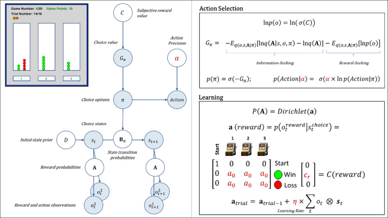
Figure 1.

Upper left: Illustration of the three-armed bandit task interface. In each of 20 games, participants had 16 opportunities (trials) to choose between one of three options with unknown (but stable) probabilities of winning vs. not winning a point (corresponding to the appearance of a green vs. red circle above the chosen option). Throughout the task, the interface displayed the game number, trial number, total points earned, and history of wins/losses for each choice within the current game (number of green and red circles above each option; see main text for more details). Left panel: Graphical depiction of the computational (partially observable Markov decision process) model used with the task (described in the main text). The values of variables in blue circles are inferred on each trial, whereas parameter values in white circles are fixed on each trial. Here, arrows indicate dependencies between variables such that observations $(o_t^m)$ for each modality m (reward and observed choice) at a time t depend on choice states (s_t) at time t, where these relationships, $p(o_t^m|s_t)$, are specified by a matrix A. States depend on both previous states and the choice of action policy (π), as specified by policy-dependent transition matrices Bπ that encode p(s_t+1|s_t, π). States at t = 1 have an initial state prior specified by a vector D. Here, D = [1 0 0 0]^T, such that the participant always started in an undecided ‘start’ state at the beginning of each trial. The probability of selecting an action policy depends on its expected free energy (Gπ), which in turn depends on the subjective reward value of making different observations (e.g., a win vs. loss) for the participant (in a vector C). These preferences are defined as a participant’s log-expectations over observations, $(o_t^m)$. As shown in the top-right panel, the values in C are passed through a softmax (normalized exponential) function, σ(), which transforms them into a proper probability distribution, and then converted into log probabilities. Top right panel: Specifies the mathematical form of the dependencies between C, Gπ, π, and a in action selection. When there is no uncertainty about states (as is true of this task), Gπ assigns higher values to actions that are expected to simultaneously maximize information gain and reward. The first term on the right corresponds to expected information gain under approximate posterior beliefs (q). Large values for this first term indicate the expectation that beliefs about reward probabilities (A) will undergo a large change (i.e., that a lot will be learned about these probabilities) given a choice of policy, due to the states and observations it is expected to generate. The second term on the right motivates reward maximization, where a high reward value corresponds to a precise prior belief over a specific observation, $p(o_t^m)$. For example, if the subjective value of a win in C were c_r = 4 (see bottom right panel), this would indicate a greater subjective reward (higher prior probability) than c_r = 2. The policy expected to maximize the probability of a win (under the associated beliefs about states, observations, and reward probabilities) is therefore favored. Because the two terms in expected free energy are subtracted, policies associated with high expected reward and high expected information gain will be assigned a lower expected free energy. This formulation entails that information-seeking dominates when reward probabilities are uncertain, while reward-seeking dominates when uncertainty is low. A softmax function, σ(), then transforms the negative expected free energies into a probability distribution over policies, such that policies with lower expected free energies are assigned higher probabilities. When actions are subsequently sampled from the posterior distribution over policies, randomness in chosen actions is controlled by an action precision parameter (a). Bottom panel: After each observation of a win/loss, learning corresponds to updating beliefs in a Dirichlet distribution (a) over the likelihood matrix A that encodes reward probabilities. Here, columns indicate (from left to right) a starting state (pre-choice) and choices 1, 2, and 3, where the rows (from top to bottom) indicate the pre-choice (no reward) observation, observing reward, or no reward. The value of a₀ – the insensitivity to information parameter – is the starting value for beliefs about reward probabilities. These beliefs always start by making up an uninformative (flat) distribution, but higher starting values (e.g., 5 vs. 0.5) effectively down-weight the information-gain term in the expected free energy – leading to an insensitivity to the need for information. The values within a (reward) are then updated based on the bottom equation, controlled by a learning rate parameter (η). For more details regarding the associated mathematics, see the main text and supplemental materials, as well as (Da Costa et al., 2020; K. J. Friston, Lin, et al., 2017; K. J. Friston, Parr, & de Vries, 2017; Smith, Friston, & Whyte, 2022). Estimated model parameters are shown in dark red.