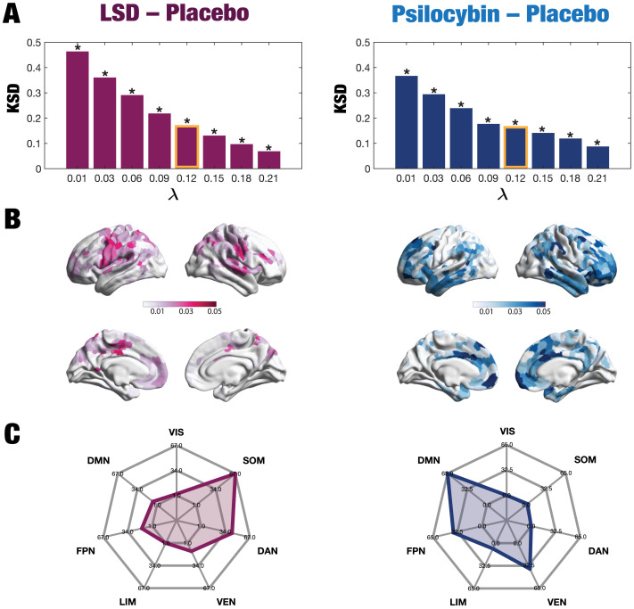
Figure 4. .

Node-level turbulence. We computed the node variability of the local synchronization defined as the standard deviation across time of the local Kuramoto order parameter. (A) The panels plot the Kolmogorov–Smirnov distance (KSD) quantifying the difference between the distributions of the node-level turbulence for each psychedelic and placebo, at each spatial scale. The smaller the KSD values, the more similar the distributions; therefore, the greatest differences were found at larger spatial scales (lower λ values). (B) The brain schemes show the absolute difference of the node-level turbulence for λ = 0.12 as an example (shown in yellow in panel A). (C) We then picked the upper 15% quantile of the absolute difference of the node-level turbulence between conditions, indexed the resting-state network to which they belong, according to Yeo’s resting-state network, and estimated the number of nodes per network. The spiderweb charts outline the number of nodes in the higher 15% quantile of the absolute difference for each comparison and network (VIS: visual; SOM: somatomotor; DAN: dorsal attention network; VEN: ventral network; LIM: limbic; FPN: frontoparietal network; DMN: default mode network). The networks that showed the most significant differences between LSD and placebo are the SOM and DAN; and between psilocybin and placebo, the FPN, DMN, and VEN. The results generalize to the other spatial scales.