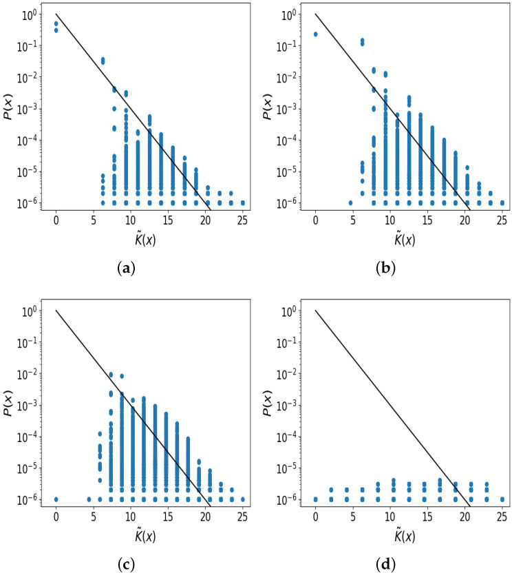
Figure 3.

Simplicity bias in the digitised logistic map from random samples with $x_0\in (0,1)$ and $\mu$ sampled in different intervals. Each blue data-point corresponds to a different binary digitised trajectory x of 25 bits in length. The black line is the upper-bound prediction of Equation (3). (a) Clear simplicity bias for $\mu \in$ (0.0, 4.0] with $P\left(x\right)$ closely following the upper bound, except for low frequency and high complexity outputs which suffer from increased sampling noise; (b) simplicity bias is still present for $\mu \in$ [3.0, 4.0]; (c) the distribution of $P\left(x\right)$ becomes more flat (less biased) and simplicity bias is much less clear when $\mu \in$ [3.57, 4.0] due to constraining the sampling to $\mu$-regions more likely to show chaos; (d) the distribution of $P\left(x\right)$ is roughly uniform when using $\mu =4.0$, with almost no bias, and hence no possibility of simplicity bias.