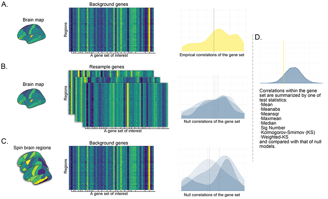
Fig. 1.

A typical gene set analysis in which researchers examine the association between a derived brain map and the transcriptomic profiles of a set of genes. A. The derived brain map is correlated with the transcriptional profiles of background genes (i.e., the 6513 available genes). The density plot illustrates the distribution of the empirical correlations for a gene set of interest. The y-axis represents the estimated probability density of observing a correlation at the x-axis. B. Competitive null models built by resampling genes. Three repetitions (i.e., iterations) are illustrated. For each repetition, the original brain map is correlated with background genes with labels shuffled. The density plots represent the resultant null distributions. C. Self-contained null models built by spinning brain regions. Three repetitions (i.e., iterations) are illustrated. For each repetition, the original background genes are correlated with the brain maps whose regions are shuffled while preserving their spatial information (i.e., spinning the brain phenotype). The density plots represent the resultant null distributions. D. The empirical correlations within a prior gene set are summarized by one of the following test statistics: Mean, Meanabs, Meansqr, Maxmean, Median, Sig Number, KS and Weighted KS, and compared against that from either competitive or self-contained null models. The yellow vertical line represents the summarized value of the empirical correlations. A total of 5000 null models are built. For each repetition, the null correlations are summarized, and the density plot shows the distribution of the summarized values of the null correlations obtained from either the competitive or self-contained null models.