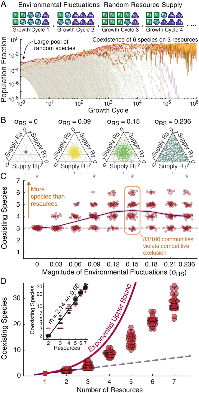
Fig 4. With environmental fluctuations, communities of random species frequently violate competitive exclusion.

(A) Top row illustrates our implementation of extrinsic environmental fluctuations by randomly sampling the resource supply fractions on each growth cycle while keeping total supply constant (Methods). Plot shows population fractions at the end of each growth cycle for an example in which 5,000 random species were inoculated and simulated for 106 growth cycles with a uniform-randomly sampled resource supply on each day (σRS = 0.236). (B) Illustration of our resource supply sampling distributions as a function of the fluctuation magnitude σRS on simplex diagrams in which an equal supply of all resources maps to the middle of the triangle and a single resource being supplied maps to a corner (Section A in S1 Text, Methods). For σRS = 0.09, 0.15, and 0.236, one thousand randomly sampled resource supplies are shown. (C) We sampled 100 communities of 5000 species competing for three resources with the metabolic constraint that the L2-norm of species’ growth rates equal 1 hr-1, simulated these communities at 9 different fluctuation magnitudes, and tallied the survivors (Methods). Points represent the number of coexisting species for each community at each fluctuation magnitude, the dashed line shows the competitive exclusion principle (one species for each of the three resources), and the solid line and shaded region provide the mean number of survivors and standard error. With even the smallest level of fluctuation 13/100 of communities violated competitive exclusion, and with fluctuations of σRS = 0.09 or larger competitive exclusion was usually violated, with a peak frequency of violations of 83/100 at σRS = 0.15. (D) We next simulated 25 random species pools for each of two through seven resources using a uniform-random resource supply (σRS = 0.236 for the three-resource case, Methods). Points represent the number of survivors in the simulations. Shown for comparison are the competitive exclusion principle (one species per resource) and the exponential upper bound (Fig 3B). Inset shows the same data on a log-log scale with a monomial best fit. The monomial was a better fit than both linear and exponential models (Section A in S1 Text).
