Pattern of ventral temporal lobe interconnections in rhesus macaques

Abstract

The entorhinal cortex (EC, A28) is linked through reciprocal pathways with nearby perirhinal and visual, auditory, and multimodal association cortices in the temporal lobe, in pathways associated with the flow of information for memory processing. The density and laminar organization of these pathways is not well understood in primates. We studied interconnections within the ventral temporal lobe in young adult rhesus monkeys of both sexes with the aid of neural tracers injected in temporal areas (Ts1, Ts2, TE1, area 36, temporal polar area TPro, and area 28) to determine the density and laminar distribution of projection neurons within the temporal lobe. These temporal areas can be categorized into three different cortical types based on their laminar architecture: the sensory association areas Ts1, Ts2, and TE1 have six layers (eulaminate); the perirhinal limbic areas TPro and area 36 have an incipient layer IV (dysgranular); and area 28 lacks layer IV (agranular). We found that (1) temporal areas that are similar in laminar architecture by cortical type are strongly interconnected, and (2) the laminar pattern of connections is dependent on the difference in cortical laminar structure between linked areas. Thus, agranular A28 is more strongly connected with other agranular/dysgranular areas than with eulaminate cortices. Further, A28 predominantly projected via feedback-like pathways that originated in the deep layers, and received feedforward-like projections from areas of greater laminar differentiation, which emanated from the upper layers. Our results are consistent with the Structural Model, which relates the density and laminar distribution of connections to the relationship of the laminar structure between the linked areas. These connections were viewed in the context of the inhibitory microenvironment of A28, which is the key recipient of pathways from the cortex and of the output of hippocampus. Our findings revealed a higher population of calretinin (CR)-expressing neurons in EC, with a significantly higher density in its lateral division. Medial EC had a higher density of CR neurons in the deep layers, particularly in layer Va. In contrast, parvalbumin (PV) neurons were more densely distributed in the deep layers of the lateral subdivisions of rostral EC, especially in layer Va, whereas the densities of calbindin (CB) neurons in the medial and lateral EC were comparable in all layers, except for layer IIIa, in which medial EC had a higher CB population than the lateral. The pattern of connections in the inhibitory microenvironment of EC, which sends and receives input from the hippocampus, may shed light on signal propagation in this network associated with diverse aspects of memory, and disruptions in neurologic and psychiatric diseases that affect this region.

Graphical abstarct

In macaques, connections are more frequent between architectonically similar ventral temporal cortices, in line with the Structural Model, which predicts density and laminar distribution of connections based on cortical type differences between linked areas. Pathways associated with memory in the entorhinal cortex are embedded in the laminar inhibitory microenvironment.

1 |. INTRODUCTION

The cortical connections between the areas of the temporal lobe are critical for memory processes.The medial temporal lobe (MTL) is implicated in episodic memory, which involves the recollection of facts and events, (Lavenex & Amaral, 2000; Squire et al., 2004) and requires encoding, consolidation, and retrieval (Sakai & Miyashita, 1993). It is thought that episodic memories are dependent on the structures within the MTL, which in turn convey information to the rest of the neocortex (Lavenex et al., 2002; reviewed in Rosene & Van Hoesen, 1987).

The MTL is composed of the hippocampal region (the CA fields, the dentate gyrus, and the subicular complex) and adjacent limbic cortices. From a medial to lateral direction, the entorhinal cortex (EC) or area 28 (A28) abuts the hippocampal region, and is continuous laterally with the perirhinal (PRC) cortices rostrally and parahippocampal (PHC) cortices caudally (Lavenex & Amaral, 2000; Squire et al., 2004). Multiple lesion and physiological studies have shown that the different cortical areas within the MTL not only send information to the hippocampus proper but are also involved in distinct aspects of memory processing (Lavenex & Amaral, 2000; Munoz & Insausti, 2005).

The MTL region is bordered laterally by unimodal sensory and multimodal association cortices. Unimodal visual areas include the inferotemporal cortices (areas TE1, TE2, TE3, TEm, and TEa). TE is the last stage of the occipitotemporal pathway involved in the processing of the features of the visual environment and their memory (e.g., Desimone & Gross, 1979; Desimone & Ungerleider, 1989; Gross et al., 1984; Suzuki & Eichenbaum, 2000). Adjacent areas on the superior temporal gyrus (STG) (areas Ts1, Ts2, and Ts3) are associated with processing of auditory signals, while several areas within the depths of the superior temporal sulcus receive convergent sensory-related pathways (Seltzer & Pandya, 1978) and also contribute projections to MTL. The perirhinal cortices (A35 and A36), found immediately lateral to EC, receive signals from unimodal visual association areas (primarily areas TE and anterior area TEO), while the parahippocampal cortices (Bonin and Bailey’s areas TF and TH) preferentially receive pathways from polymodal association areas and posterior visual areas (Lavenex & Amaral, 2000; Suzuki & Amaral, 1994b). These high-order sensory association cortices transmit signals via sequential corticocortical pathways to MTL areas, which reach the hippocampus mostly via the EC. The EC receives the majority of its input from the PRC and PHC and transmits these complex multisensory-related signals to areas within the hippocampal region through the perforant pathway. Signals from these pathways, along with those from subcortical structures, are thought to help integrate the external cues with the internal states for memory encoding (Van Hoesen et al., 1972).

In the reverse direction, projections from the hippocampal region reach A28 as well as PRC and PHC and from there nearby MTL areas and high-order association and sensory cortices. The PRC and PHC are largely involved in reciprocal connections with other cortical areas in the temporal, insular, frontal, cingulate, retrosplenial, and parietal cortices (Suzuki & Amaral, 1994a). These output-related pathways are thought to be involved in memory consolidation (Lavenex & Amaral, 2000; Munoz & Insausti, 2005).

The EC thus has a unique position in MTL as recipient of the extensive flow of signals from the cortex via pathways from adjacent perirhinal and parahippocampal areas and transmitting hippocampal output to the rest of the cortex. In macaque monkeys, the EC is a complex region, subdivided into seven parts based on cytoarchitecture and connections (Amaral et al., 1987; Munoz & Insausti, 2005).

The interconnections of MTL and their presumed feedforward and feedback nature have been studied in classical studies (e.g., Suzuki & Amaral, 1994b), but several issues pertaining to their organization remain unresolved. First, in view of the fact that the MTL is composed of areas that have distinct architecture (Amaral et al., 1987), to what extent is the density of the connections associated with the diverse types of cortices? In MTL, cortical types range from the agranular A28 and A35 to dysgranular medial A36 in the PRC, to granular areas of lateral A36 and adjacent six-layered (eulaminate) sensory and high-order association cortices. Second, to what extent are the interconnections reflected in their laminar distribution based on the relative difference in the architecture of pairs of linked areas, as proposed (Barbas & Rempel-Clower, 1997)? Finally, since EC is the gateway to hippocampus as well as a main relay from the hippocampus to the cortex, what is the composition of the inhibitory microenvironment within EC, which likely is critical in the processing from these pathways?

To address these issues, we used neural tracers to study the origin of projection neurons that interlink MTL areas and some adjacent sensory association cortices. In addition, we addressed the inhibitory microenvironment of A28, which sits at the center of the flow of signals to and from the hippocampus, by studying the distribution of three neurochemical classes of inhibitory neurons in the anterior EC–calretinin (CR), parvalbumin (PV), and calbindin (CB), which are calcium-binding proteins that are expressed in largely nonoverlapping functionally distinct types of inhibitory neurons (DeFelipe, 1997). Together, these neurochemical classes account for most of the inhibitory neuronal population in the primate cortex (reviewed in DeFelipe, 1997). We focused on the anterior half of EC for the study of CR, PV, and CB neurons largely because it included the bulk of the connections from our injection sites. The anterior EC is also strongly connected with medial prefrontal cortices in the anterior cingulate and orbitofrontal cortices. These pathways are at the confluence of complex processing for context, emotion, cognition, and memory (reviewed in Barbas, 2015), in processes where inhibitory neurons play a key role (Bunce & Barbas, 2011; Bunce et al., 2013; reviewed in Anderson et al., 2015; Barbas et al., 2013). Our results reveal a complex but systematic linkage of MTL interconnections to the type of cortices involved in the projection system.

2 |. METHODS

2.1 |. Surgery, tracer injection, and tissue processing

We conducted experiments on nine rhesus monkeys (Macaca mulatta, 2–5.5 years, n = 3 female) for tracing, architectonic parcellation, and photography (Table 1), according to the ILAR Guide for the Care and Use of Laboratory Animals (publication 80–22 revised, 1996). Animal protocols were approved by the Institutional Animal Care and Use Committee at Boston University School of Medicine and Harvard Medical School. Experimental procedures were designed to minimize animal suffering. We placed multiple distinct tracers in each case, which we used for this and other unrelated studies so as to reduce the number of animals needed for research.

TABLE 1.

List of cases and analyses performed.

Case	Sex	Age (years)	Hemisphere	Injection site	Tracer	Analysis
AN	–	–	Right	NA	NA	Nissl, myelin, SMI-32
AT	Female	2	Right	A36	BDA	Retrograde
AT	Female	2	Right	TE1	FB	Retrograde
AT	Female	2	Right	TPro	DY	Retrograde
AV	–	–	Left	TE1/Ts1	BDA	Retrograde
BC	Male	–	Right	STG	FR	Retrograde
BD	Male	–	Right	NA	NA	Photomicrographs for CB and PV
BS	Female	3.5	Right	NA	NA	Stereology in a28 for CB, CR, and PV
BV	Male	4	Right	NA	NA	Stereology in a28 for CB, CR, and PV
BW	Female	5.5	Right	NA	NA	Stereology in a28 for CB, CR, and PV; photomicrographs for CR
MMR	Male	–	Left	A28	Tritiated amino acids; mixture of tritiated leucine and proline	Anterograde

Abbreviations: BDA, biotinylated dextran amine; CB, calbindin; CR, calretinin; DY, Diamidino Yellow; FB, Fast Blue; FR, Fluoro-Ruby; PV, parvalbumin.

We first obtained high-resolution magnetic resonance imaging (MRI) scans of the brain in vivo for surgical planning. Animals were first sedated with ketamine hydrochloride (10–15 mg/kg, i.m.), anesthetized with propofol (loading dose 2.5–5 mg/kg, i.v.; continuous infusion rate 0.25–0.4 mg/kg/min), and placed in a stereotaxic apparatus (1430 M; David Kopf Instruments). We used MRI scans to calculate stereotaxic coordinates using the interaural line as reference for injection of neural tracers.

We performed surgery under general anesthesia (isoflurane, to a surgical level) with continuous monitoring of vital signs. We injected one or three tracers in each monkey, as shown in Table 1. The dyes injected included Fast Blue (FB; case AT, 3% dilution, 2 μL; Polysciences), biotinylated dextran amine (BDA; cases AV and AT: equal parts 10% 10 kDA and 10% 3 kDA, 5 μL; Invitrogen), Diamidino Yellow (DY; case AT, 3% dilution, 4 μL), and Fluoro-Ruby (FR; case BC, 10% solution, mixture of 10 kDA and 3 kDA, 4 μL; Invitrogen). The 10-kDA dextran amine (BDA, FR) variant is optimal for labeling axonal projections and their terminations, while the 3-kDA variant is optimal for retrograde labeling of cell bodies and proximal dendrites (Reiner et al., 2000; Richmond et al., 1994; Veenman et al., 1992). To avoid dye leakage along the needle trajectory, we loaded needles with a small bubble of air after aspiration of the dye and left the syringe at the site of injection for 5–10 min to allow local diffusion and prevent backward suction of the dye during needle withdrawal. We monitored animals postoperatively and gave antibiotics and analgesics.

After a survival period of 18–20 days, the animals were anesthetized with a lethal dose of sodium pentobarbital (~50 mg/kg, i.v., to effect) and perfused transcardially with 4% paraformaldehyde and 0.2% glutaraldehyde in 0.1 M PB, pH 7.4 (cases BC, BS, and BV) or 4% paraformaldehyde in cacodylate buffer or in 0.1 M PB at pH 7.4 (cases AN, AT, AV, and BW). The brains were removed, photographed, cryoprotected in ascending concentrations of sucrose solutions (10%–25% sucrose in 0.1 M PB, pH 7.4, with 0.05% sodium azide; Sigma–Aldrich), frozen in −80°C isopentane (Rosene et al., 1986), and sectioned on a freezing microtome (AO Scientific Instruments/Reichert Technologies) in 50-μm coronal sections (40 μm for cases AN, AT, and AV). Sections were collected into 10 matched series and stored in antifreeze (30% ethylene glycol, 30% glycerol, 0.05% sodium azide in 0.05 M phosphate buffer, pH 7.4). One of the 10 series was mounted directly from the microtome blade onto gelatin-coated slides and placed in cold storage (4°C) for mapping labeled neurons directly using epifluorescence, as described previously (Barbas et al., 2005).

We also used an archival case (MMR) with a purely anterograde tracer (tritiated amino acids) injected in the medial part of the anterior EC (tritiated amino acids, New England Nuclear, L-2,3-[3H]proline, 35 Ci/mmol and L-3,4,5-[3H]leucine, 80 Ci/mmol), and processed for autoradiography, as described previously (Aggleton et al., 2015; Kosel et al., 1982; Saunders & Rosene, 1988). The surgical procedure in this case followed a basal approach after positioning the head in a different head holder that fixed the eye socket and head and allowed rotation of the head in three planes (Aggleton et al., 2015; Saunders & Rosene, 1988). After a survival period of 7 days, the animals were anesthetized with a lethal dose of sodium pentobarbital (~50 mg/kg, i.v., to effect) and perfused transcardially with 4% paraformaldehyde. The brains were then stored in 10% formalin for 2 weeks, and subsequently embedded in paraffin and cut into 10-μm serial coronal sections, as described previously (Aggleton et al., 2015; Saunders & Rosene, 1988). Sections were mounted on glass slides coated with Kodak NTB2 emulsion, stored at 4°C in the dark, and subsequently processed using a method modified from Cowan et al. (1972). Mounted sections were stored between 6 and 12 weeks prior to development and subsequent Nissl staining, as described previously (Blatt & Rosene, 1998; Rosene & Van Hoesen, 1977).

2.2 |. Visualization and imaging of markers of interest

To visualize projection neurons labeled by tracers, we incubated free-floating sections for 1 h at 4°C in 0.05 M glycine (Sigma–Aldrich) and preblocked for 1 h at 4°C in 5% normal goat serum (NGS; Vector Laboratories), 5% bovine serum albumin (BSA; Sigma–Aldrich), and 0.2% Triton-X (Sigma–Aldrich) in 0.01 M PBS. For cases using BDA tracer (AT, AV), sections were incubated for 1 h at 25°C with avidin-biotin horseradish peroxidase (AB-HRP; Vectastain Elite ABC kit, Vector) at a 1:100 dilution in PBS, followed by three rinses in PBS (10 min each), and tracer was visualized with incubation for 1–3 min in diaminobenzidine (DAB substrate kit, Vector).

Sections were then mounted on gelatin-coated glass slides, dried, counterstained with Nissl (thionin stain, every other section) as previously described (García-Cabezas et al., 2016), and coverslipped with Entellan (Sigma–Aldrich). In the cases with injection of FB and DY, sections were mounted immediately after cutting, dried, and coverslipped with Krystalon (Millipore); labeled neurons were mapped directly using a microscope with epifluorescence illumination, as described previously (Barbas et al., 2005; Xiao et al., 2009).

Sections used to visualize neurons retrogradely labeled for tracers (FB, DY, or FR) were viewed under a microscope with epifluorescence attachment (Nikon Optiphot) that includes an analog–digital microscope/computer interface (Nikon, Optiphot/Austin) for mapping and counting labeled neurons and axon terminals with custom-made software that was developed in our laboratory.

To process tissue for architectural markers used to further aid cortical parcellation, and for photography (AT, AV, BC), full series were stained with thionin, myelin (Gallyas, 1979; Garcia-Cabezas et al., 2017; Zikopoulos et al., 2016), or an antibody for SMI-32 (mouse monoclonal, 1:5000, BioLegend, RRID: AB_10719742) (Garcia-Cabezas et al., 2022; John et al., 2022).

For brightfield photography, we used an Olympus optical microscope (BX51) with a CCD camera (Olympus DP70) connected to a commercial imaging system (DP Controller, Olympus). Figures were assembled in Adobe Illustrator CC software (RRID: SCR_010279). Brightness, contrast, and saturation adjustments were made overall without retouching, using Adobe Photoshop (RRID: SCR_014199) and/or ImageJ (RRID: SCR_003070) (Rasband, 1997–2014).

To view inhibitory neurons (PV, CB, or CR; cases BS, BV, and BW), we used single labeling immunohistochemistry. Free-floating sections were rinsed in 0.1 M PB and incubated in 0.01 M sodium citrate buffer (pH 8.5, 80°C, 30 min) for antigen retrieval (Jiao et al., 1999), and then incubated in 0.05 M glycine (4°C, 1 h) to bind free aldehydes, and then in 0.3% H₂O₂ in 0.01 M PBS (30 min) to quench endogenous peroxidases. We preblocked sections (1 h, 4°C) in 10% normal goat serum (NGS; Vector Laboratories), 5%–10% bovine serum albumin (BSA; Sigma–Aldrich), 0.2% BSA-c (Aurion), and 0.2%–0.4% Triton-X-100 (Sigma–Aldrich) in 0.1 M PB. For immuno-labeling of local inhibitory interneurons, we incubated the sections for 3 days with primary antibodies against calcium-binding proteins (mouse anti-PV [Swant, catalog #235, RRID: AB_10000343], mouse anti-CB [Swant, catalog #300, RRID: AB_10000347], mouse anti-CR [Swant, catalog #6B3, RRID: AB_10000320]). We then used a biotinylated secondary antibody (1:200 in 1% NGS, 1% BSA, 0.2% Triton X-100; goat anti-mouse, IgG; Vector Laboratories, catalog #BA-9200, RRID: AB_2336171) and later we incubated the sections in avidin-biotin horseradish complex (ABC, Vector, catalog #PK-6100, RRID: AB_2336819). The sections were later processed with diaminobenzidine (DAB substrate kit, Vector, catalog #SK-4100, RRID: AB_2336382) as described previously (Barbas et al., 2005; Liu et al., 2020).

2.3 |. Architectonic borders and nomenclature

To place architectonic borders, we used Nissl-counterstained sections (thionin) from each mapped series. We used several maps to determine architectonic boundaries for MTL and other temporal regions. For medial temporal areas (areas 28, 35, 36, TH, TF), we relied on maps from previous studies (Amaral et al., 1987; Saleem et al., 2007; Suzuki & Amaral, 2003) with some modifications. We subdivided TF into medial and lateral regions for the anterograde injection in A28. We adhered to temporal pole nomenclature as previously described (Hoistad & Barbas, 2008; Rempel-Clower & Barbas, 2000). We parcellated the STG and superior temporal sulcus (STS) according to previous maps (Barbas et al., 1999; Galaburda & Pandya, 1983; Medalla & Barbas, 2014; Pandya & Sanides, 1973; Seltzer & Pandya, 1978), as elaborated for each region below.

2.3.1 |. Temporal polar cortices

We employed the terminology used in previous studies (Hoistad & Barbas, 2008; Rempel-Clower & Barbas, 2000), which was adapted from several studies and later modified. The temporal pole was divided into the agranular temporal periallocortex (TPall), the dysgranular dorsomedial temporal pole (TPd), and the dysgranular ventromedial temporal pole (TPv). The granular areas of the temporal pole are laterally located and consist of the auditory association areas Ts1 and Ts2 and the anterior region of the visual association area TE1.

2.3.2 |. MTL cortices

We divided the EC according to Insausti and Amaral and followed their nomenclature: E_O (olfactory), E_R (rostral), E_LR (lateral rostral), E_I (intermediate), E_LC (lateral caudal), E_C (caudal), and E_CL (caudal-limiting) based on cytoarchitecture (Amaral et al., 1987). The perirhinal cortical area 35 included the cortex in the depths of the rhinal sulcus. We subdivided A36 into four parts—rostromedial (rm), rostrolateral (rl), caudomedial (cm), and caudolateral (cl)—but summarized the data into medial and lateral regions. A35 was parcellated according to Lavenex et al. (2002), and the divisions of A36 followed the nomenclature employed in previous studies, starting with the appearance of the rhinal sulcus (Lavenex et al., 2002). The parahippocampal cortical areas were based on previous maps (Lavenex et al., 2002; Suzuki & Amaral, 1994b), which divided the PHC into Bonin and Bailey’s areas TH and TF (Suzuki &Amaral, 1994a).

2.3.3 |. Cortices in the lateral region of the temporal lobe

The parcellation of the lateral temporal areas was based on previous literature by Pandya and colleagues, as modified from Brodmann’s map (Pandya & Sanides, 1973; Seltzer & Pandya, 1978). We divided the areas in the STG, ventral to the lateral sulcus (ls) and dorsal to the superior temporal sulcus (sts), according to the map of Pandya and Sanides (1973). The auditory region was parcellated into the medial and lateral koniocortex, prokoniocortex area (proA), parakoniocortex caudal (paAc), parakoniocortex lateral (paAlt), and parakoniocortex rostral (paAr); its adjacent areas were divided into parainsular (PaI), retroinsular temporal (reIt), temporoparietal (Tpt), and temporalis superior 1, 2, and 3 (Ts1, Ts2, and Ts3) (Pandya & Sanides, 1973). The areas on the dorsal bank of the superior temporal sulcus were parcellated into TAa, TPO, and PGa, according to the map of Seltzer and Pandya (1978).

2.3.4 |. Cortices in the inferior region of the lateral temporal lobe

The region ventral to the superior temporal sulcus and lateral to A36 (anteriorly) and to the occipitotemporal sulcus (ots) (posteriorly) was labeled as TE by Bonin and Bailey, which Seltzer and Pandya later subdivided into five distinct areas: TE1, TE2, TE3, TEm, and TEa (Seltzer & Pandya, 1978). IPa is located at the depths of the ventral bank of the superior temporal sulcus, found medial to TEa (Seltzer & Pandya, 1978).

2.3.5 |. Insular cortices

We divided the insular cortex into granular (Ig), dysgranular (Idg), and agranular (Iag) regions.

2.4 |. Pathway mapping and data analysis

We used exhaustive plotting to map cortical pathways directed to distinct MTL areas in a series of coronal sections through the MTL region and in adjacent inferior temporal (visual) and superior temporal (auditory) association and multimodal areas in the depths of the superior temporal sulcus. We mapped a series of sections (one in 20 sections) through the ipsilateral hemisphere. In each series, we mapped all labeled cortical neurons at 200× using brightfield or epifluorescence microscopy using a semiautomated commercial system (Neurolucida, RRID: SCR_001775; Olympus BX60). Labeled neurons were included in one of two laminar categories: superficial (layers II and III) or deep (layers V and VI), according to the lower boundary of layer III (for FB or DY, this was done after mapping and counterstaining with Nissl).

We computed the number of labeled neurons in a specific area as a proportion of the total labeled neurons in the temporal lobe. This normalization approach allowed each case to be its own control, in view of likely variation across cases in the size of injection sites, tracer transport dynamics, and immunolabeling, even when identical procedures are used. To describe the laminar distribution of labeled neurons within and across cases, we aggregated labeled neurons across sections for each cortical area in each case. We expressed laminar specificity as the percent of labeled neurons originating in the upper layers (II and III), referred to as the supragranular index (SGI), which was calculated for areas with ≥1% of labeled neurons. Percentages were averaged across cases and expressed with standard error of the mean. We analyzed data from each case separately to test the consistency of the findings. We used MATLAB (RRID: SCR_001622) to obtain the z-scores of the normalized density of all connections and with these values we created a matrix, which we then color coded by using MATLAB’s heatmap feature. We used the heatmap feature to color code the matrix that shows the SGI per temporal area of origin directed to each of the injection sites (Ts2, Ts1/TE1, TE1, TPro, and A36).

We studied case MMR (anterograde tracer injection in A28) by analyzing the efferent projections from A28 to other temporal areas using ImageJ (Rasband, 1997–2014). For brightfield and darkfield photography, we used an Olympus optical microscope (BX53) with a CCD camera (Olympus DP74) connected to a commercial imaging system (DP Controller, Olympus). In ImageJ, we used the auto threshold feature and the moments method to analyze the images. We found this method to be the one that best represented the signal of the tracer. We used the binary images to obtain the measurement for area fraction, which is the area of the image that was occupied by the signal. We acquired the area fraction measurement for the column (width of 150 μm and height differed among areas) with the highest intensity within each area. We then computed the proportion of area fraction of each area of the temporal lobe by dividing the measurement recorded per area over the total amount of area fraction measured in this case.

2.5 |. Mapping putative inhibitory neurons labeled with PV, CB, and CR

To map the distribution of labeled neurons by layer, we used stereology and the optical fractionator method via a semiautomated commercial system (Stereoinvestigator, RRID: SCR_002526; Olympus BX63). The optical fractionator method extrapolates a density for the region of interest based on section thickness and systematic sampling at regular intervals (Howard & Reed, 1998). We used a grid size of (250 μm²), a counting frame of (225 μm²), and a disector height of 5 μm with a guard zone of 2 μm at the top and bottom of each section. This sampling rate yielded a coefficient of error at or below 10%, as recommended previously (Gundersen, 1986). We systematically sampled the medial and lateral divisions of the anterior region of EC in three coronal sections spaced 20 or 40 sections apart, depending on the case. We computed the density separately for laminar groups, and expressed data as the population of labeled neurons in the superficial layers (I–-III), deep layers (lamina dissecans [LD]—layer VI), and all layers (I–VI). The densities of each inhibitory neurochemical neuronal class were averaged across cases (BS, BV, BW) and expressed with standard error of the mean. We used a one-way ANOVA to compare the laminar distribution of inhibitory neuronal subpopulations between the lateral and medial subdivisions of the EC. Significance was set at p = .05. Descriptive statistics and analyses were performed using MATLAB (RRID: SCR_001622).

2.6 |. Statistical analysis of laminar data

We averaged the percent of neurons in the superficial layers across cases for each pathway direction. We also performed linear regressions to test if cortical type difference of connected areas is correlated with the proportion of neurons found in the superficial layers. Specifically, for area with labeled neurons in each case, we calculated the cortical type difference between the area of origin and area of termination (the injection site of retrograde tracers) and conducted linear regression analyses between SGI and cortical type difference (Barbas, 1986; Barbas & Rempel-Clower, 1997). Regressions were performed by cortical type on cortical areas pooled across cases and for each case separately to study individual variability.

2.7 |. Controls

In immunohistochemical protocols, we omitted primary antibodies in control sections of tissue and found no labeling. We excluded some areas because they were close to injection site for the laminar analysis only, where some labeled neurons could have been labeled by tracer to nearby sites within the same area as the injection site.

3 |. RESULTS

3.1 |. Systematic variation of the cortex

Beyond the maps of individual areas used for our initial qualitative analysis of laminar densities and cytoarchitecture (above), we classified areas into cortical types in the context of the fundamental principle of graded systematic variation of cortical lamination and structure. This principle was discovered independently by different investigators working with different species and on different continents (e.g., Abbie, 1940, 1942; Dart, 1934; Sanides, 1969; von Economo, 1927/2009). In the context of this classical principle, systematic variation in laminar structure in MTL and adjacent areas of the temporal lobe is seen along the mediolateral and the rostrocaudal axes. Beyond the limbic ring of the hippocampal region, cortical lamination becomes progressively more distinct (reviewed in Barbas, 2015; Garcia-Cabezas et al., 2019). Figure 1 shows a schematic of cortical types in the temporal lobe. The simplest structural type is “agranular,” which describes areas that lack layer IV. Dysgranular includes areas that have an incipient layer IV. Eulaminate areas have six cortical layers, but they can vary by the thickness of layer IV as well as the distinction of the other layers and distribution of various cellular and molecular markers.

FIGURE 1.

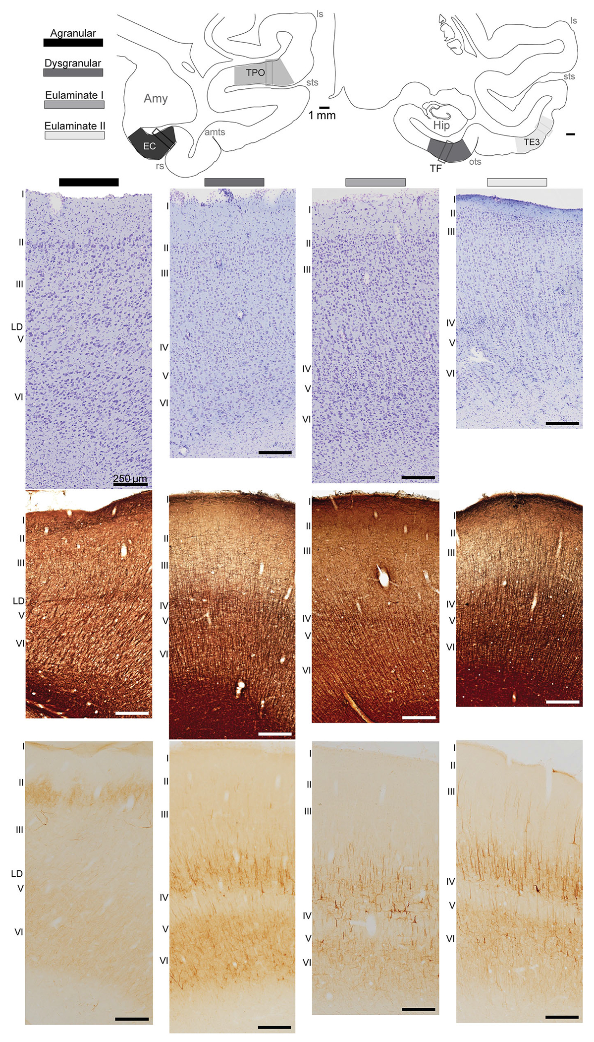
Cortical types within the temporal lobe. The gradient from agranular (black) to eulaminate II (light gray) represents the gradual change in cortical type in the mediolateral axis of the cortex. Schematic of coronal sections shows locations of representative areas from each cortical type, with boxes delineating from where photomicrographs were obtained (top). Photomicrographs show Nissl (top), myelin (middle), and SMI-32 (bottom) labeling from representative agranular, dysgranular, eulaminate I, and eulaminate II areas. Laminar labels: I, II, III, lamina dissecans (LD), V, and VI. amy, amygdala; amts, anterior middle temporal sulcus; hip, hippocampus; ls, lateral sulcus; ots, occipitotemporal sulcus; rs, rhinal sulcus; sts, superior temporal sulcus.

One example of a reliable architectonic marker in the primate cortex is the antibody for the intermediate neurofilament protein SMI-32, which labels the soma and dendrites of a subpopulation of pyramidal neurons found primarily in the deep part of layer III and the upper part of layer V, and to a lesser extent in layers II, Vb, and VI (Campbell & Morrison, 1989; Garcia-Cabezas et al., 2022; John et al., 2022). Layer IV is devoid of SMI-32 label. As seen in representative columns through the temporal lobe areas in Figure 1, expression of SMI-32 increases in areas along the mediolateral axis, as the cortical lamination becomes more elaborate. It is also evident that the laterally located eulaminate areas have a higher concentration of myelin than the agranular and dysgranular cortices (Figure 1).

The above qualitative analysis of structural architectonic markers reveals that even though there are many cortical areas, they can be classified by cortical type across the cerebral cortex (reviewed in Barbas, 2015; Garcia-Cabezas et al., 2019). In the context of this principle, we have classified MTL and adjacent areas with injection sites into cortical types as follows: Agranular—A28; Dysgranular—rostromedial A36 and TPro; Eulaminate I—TE1, Ts1/TE1, and Ts2. We then quantified the density and laminar distribution of neurons that interlink these areas and assessed how connection patterns relate to differences in cortical type.

3.2 |. Injection sites of neural tracers

One injection was in area Ts2 (FR), another in Ts1/TE1 (BDA), another in TE1 (FB), another in TPro (DY), another in A36 (BDA), and finally an injection of the anterograde tracer ³H amino acids was in EC (A28). The details of these cases are listed in Table 1. Most of these cases were used previously for studies unrelated to the present.

3.3 |. Density of connections

We first studied connections within the temporal lobe by quantitative study of projection neurons after injection of retrograde or bidirectional tracers in different areas of the temporal lobe:Ts1,Ts2,TE1,A36, and TPro. These areas can be categorized into two different cortical types based on their architecture. Ts1, Ts2, and TE1 have six layers, and thus are known as eulaminate, while A36 and TPro are dysgranular, characterized by an ill-defined layer IV. For each of the injections, we mapped quantitatively the retrogradely labeled neurons in cortical areas of the temporal lobe and calculated the proportion of projection neurons within each of the temporal areas for all labeled neurons in the temporal lobe in each case.

3.4 |. Distribution of the projection neurons directed to Ts2

Most projection neurons directed to Ts2 (Figure 2a) emanated from other eulaminate areas (Figure 2b–e). As shown in Figure 2f, Ts2 received projections largely from nearby areas within Ts2, and from areas TPO, TAa, TPro, PaI, and TPall, with each area contributing at least 10% of the total number of neurons directed to it. Areas Ts3, PGa, and TF each made up more than 1% of the neurons projecting to this area. In contrast, only sparse labeled neurons were directed to Ts2 from A35, TH, A28, TPd, TPv, A36, Idg, proA, Ts1, TEm, TE1, TEa, IPa, TAa, and paAlt (Figure 2f).

FIGURE 2.

Distribution of projection neurons directed to superior temporal cortical area Ts2. (a) The injection site of fluororuby in the STG area Ts2. (b–e) Projection neurons (pink dots) were mapped from coronal sections from anterior (b) through posterior (e) levels of the temporal lobe. The dotted line shows the upper part of layer V. (f) Proportion of labeled neurons in distinct architectonic areas as a fraction (%) of all labeled neurons found in the temporal lobe in this case. amy, amygdala; amts, anterior middle temporal sulcus; hip, hippocampus; ls, lateral sulcus; ots, occipitotemporal sulcus; rs, rhinal sulcus; sts, superior temporal sulcus.

3.5 |. Distribution of projection neurons directed to Ts1/TE1

Labeled neurons directed to Ts1/TE1 (Figure 3a) were found in multiple areas within the temporal lobe, mostly in other eulaminate areas (Figure 3b–e). More than 10% of the projection neurons directed to Ts1/TE1 emanated from areas TPO, TE1, and Ts1. Projection neurons in the range of 1%–10% were found in A36, Ts2, TAa, TEm, TEa, TE2, and IPa (Figure 3f), which are all eulaminate with the exception of A36, which has a dysgranular architecture medially and eulaminate architecture laterally; the majority of labeled neurons directed to the site of the dye injection were found in the lateral, the eulaminate part of A36. Lastly, each of areas TPall,TH, A35, EC, TPro, TF, Idg, and Ts3 included fewer than 1% of labeled neurons projecting to Ts1/TE1.

FIGURE 3.

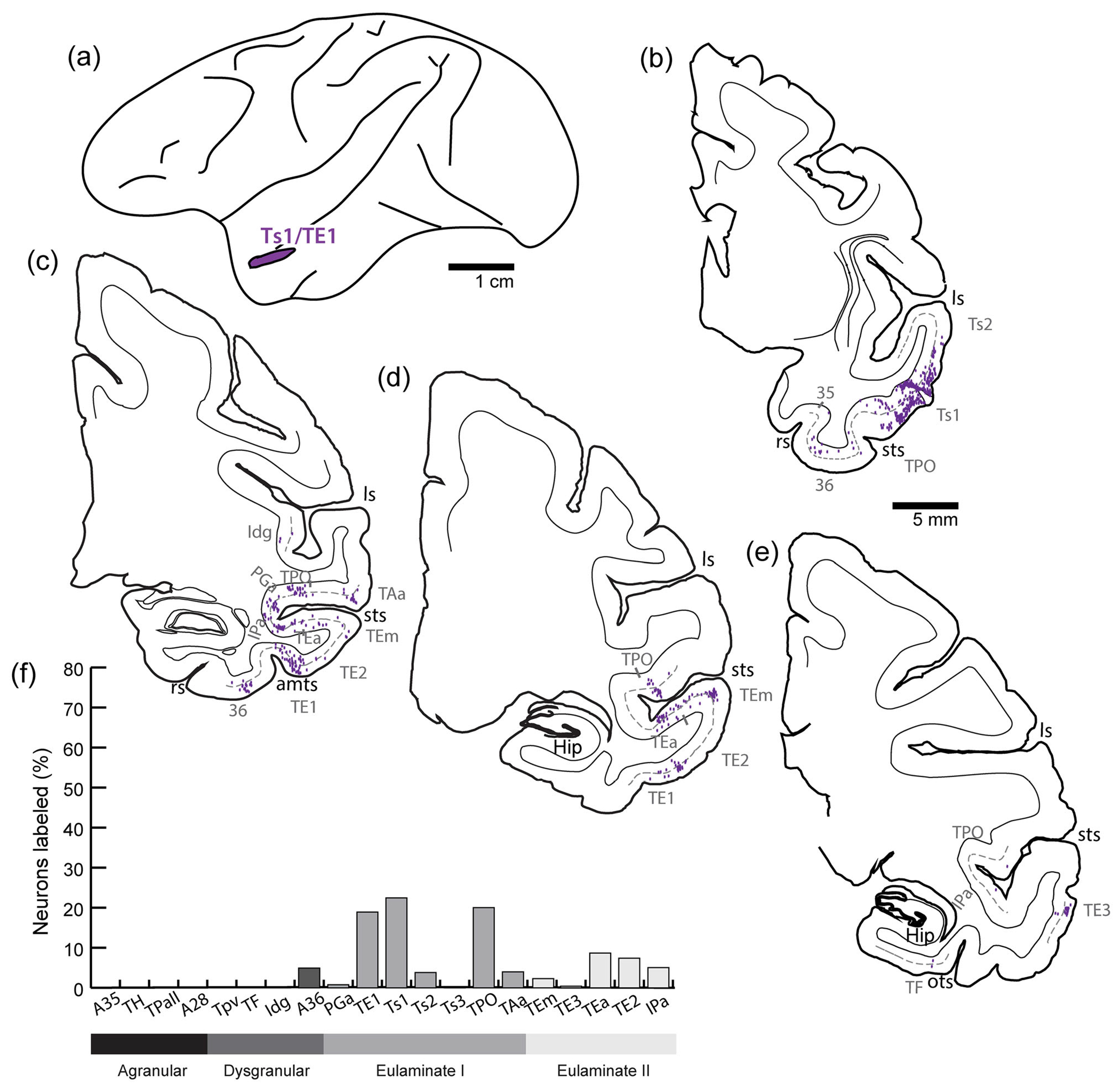
Distribution of projection neurons directed to temporal cortical areas Ts1/TE1. (a) The injection site of biotinylated dextran amine (BDA) in Ts1/TE1. (b–e) Projection neurons (purple dots) were mapped from coronal sections from anterior (b) through posterior (e) levels of the temporal lobe. The dotted line shows the upper part of layer V. (f) Proportion of labeled neurons in distinct architectonic areas as a fraction (%) of all neurons found in the temporal lobe in this case. amts, anterior middle temporal sulcus; hip, hippocampus; ls, lateral sulcus; ots, occipitotemporal sulcus; rs, rhinal sulcus; sts, superior temporal sulcus.

3.6 |. Distribution of projection neurons directed to TE1

Figure 4 shows the distribution of labeled neurons projecting to area TE1 (Figure 4a) on maps of coronal sections (Figure 4b–e). As shown in Figure 4d, most labeled neurons were distributed in A36 and TEa. In contrast, TE1 received fewer (<10%) projections from each of areas 35, 28, TF, PGa, Ts1, Ts2, and IPa. Sparse distributions of labeled neurons were found in areas Iag, TH,TPall,TPd, and TE3.

FIGURE 4.

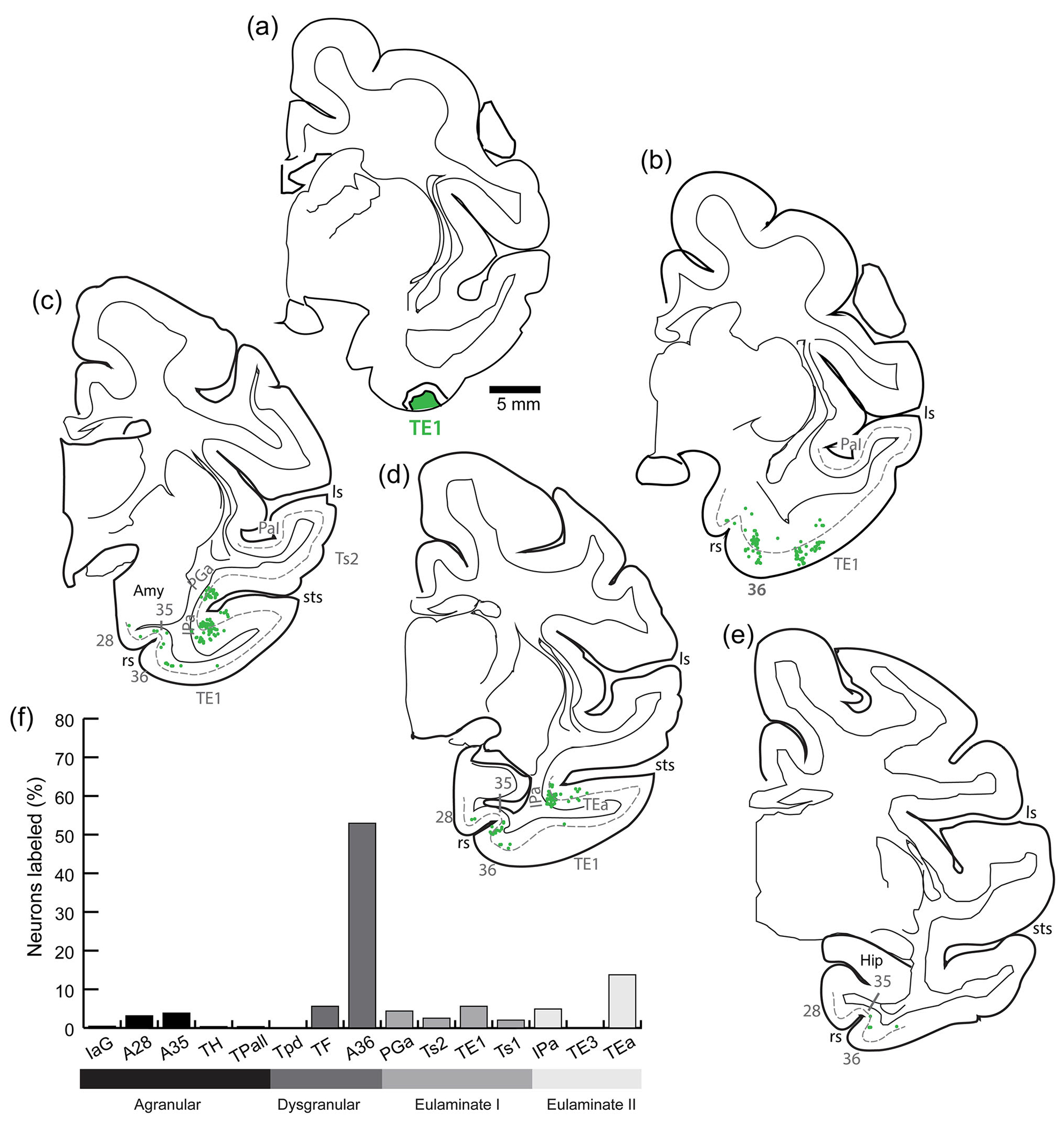
Distribution of projection neurons directed to inferior temporal cortical area TE1. (a) The injection site of fast blue in TE1. (b–e) Projection neurons (green dots) were mapped from coronal sections from anterior (b) through posterior (e) levels of the temporal lobe. The dotted line shows the upper part of layer V. (f) Proportion of labeled neurons in distinct architectonic areas as a fraction (%) of all neurons found in the temporal lobe in this case. amy, amygdala; hip, hippocampus; ls, lateral sulcus; rs, rhinal sulcus; sts, superior temporal sulcus.

3.7 |. Distribution of projection neurons directed to TPro

Most projection neurons directed to TPro (Figure 5a) originated from dysgranular areas (Figure 5b–e) in the temporal pole (TPro, TPd, TPv) and from Ts1. Other cortical areas in the temporal lobe (A35, A28, Ts2, and TE1) accounted for more than 1% of the total number of projection neurons directed to TPro (Figure 5f). Sparsely distributed labeled neurons were found in areas TPall, A36, and TEa.

FIGURE 5.

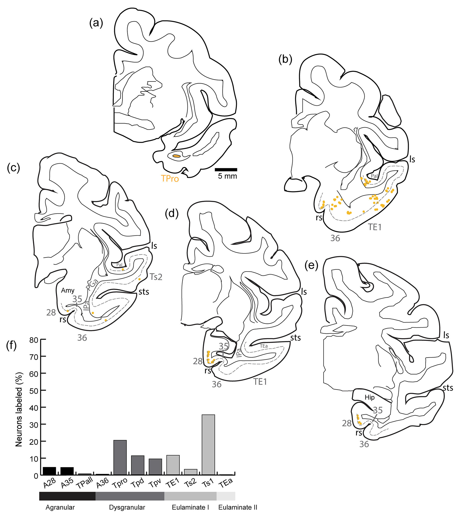
Distribution of projection neurons directed to temporal cortical area TPro. (a) The injection site of diamidino yellow in TPro. (b–e) Projection neurons (yellow dots) were mapped from coronal sections from anterior (b) through posterior (e) levels of the temporal lobe. The dotted line shows the upper part of layer V. (f) Proportion of labeled neurons in distinct architectonic areas as a fraction (%) of all neurons found in the temporal lobe in this case. amy, amygdala; hip, hippocampus; ls, lateral sulcus; rs, rhinal sulcus; sts, superior temporal sulcus.

3.8 |. Distribution of the projection neurons directed to A36

The injection of A36 was in its rostromedial (rm) region (Figure 6a). As shown in Figure 6b–e, projection neurons directed to A36rm were distributed largely in other parts of A36 and TE1, which included >10% of the total in each case. Labeled neurons in the range of more than 1% and fewer than 10% of the total projection neurons were found in A35, Ts1, A28, and TPv (Figure 6f). Lastly, A36rm received projections from only a few labeled neurons (<1% of the total) from areas TPall, Iag, Idg, PaI, PGa, Ts2, TPO, TEm, TAa, and TE2.

FIGURE 6.

Distribution of projection neurons directed to perirhinal area 36. (a) The injection site of biotinylated dextran amine (BDA) in A36. (b–e) Projection neurons (brown dots) were mapped from coronal sections from anterior (b) through posterior (e) levels of the temporal lobe. The dotted line shows the upper part of layer V. (f) Proportion of labeled neurons in distinct architectonic areas as a fraction (%) of all neurons found in the temporal lobe in this case. amy, amygdala; hip, hippocampus; ls, lateral sulcus; rs, rhinal sulcus; sts, superior temporal sulcus.

3.9 |. Distribution of axon terminations of A28

We made some additional observations on the distribution of axon terminations in an archival case with injection of the purely anterograde tracer tritiated amino acids injected along the intermediate region of EC (E_I; Figure 7a). We analyzed the efferent terminations from this site using ImageJ to compute the percent area fraction density of signal in areas of the temporal lobe. As shown in Figure 7b, terminations from area E_I were found primarily in perirhinal areas 35 and 36 and in parahippocampal areas TH and TF. Based on the injection in the intermediate part of E_I, our findings align with the findings of Suzuki and Amaral (1994b). We found that the EC projected to the medial (dysgranular) part of A36 more strongly than it did to the lateral eulaminate region of A36, which is also consistent with previous findings (Suzuki & Amaral, 1994b). Likewise, the connections between the EC and the parahippocampal areas showed the same gradient previously described (Suzuki & Amaral, 1994b). Area E_I showed strong projections to area TH, which is consistent with earlier ablation–degeneration findings (Van Hoesen et al., 1972). By contrast, its efferent projections to the lateral region of TF were less prominent than those to the medial part. Terminations were sparse in eulaminate areas (I and II), except for A36, which has a dysgranular part medially and a granular part laterally, and in which terminations from the EC were substantial (Figure 7a).

FIGURE 7.

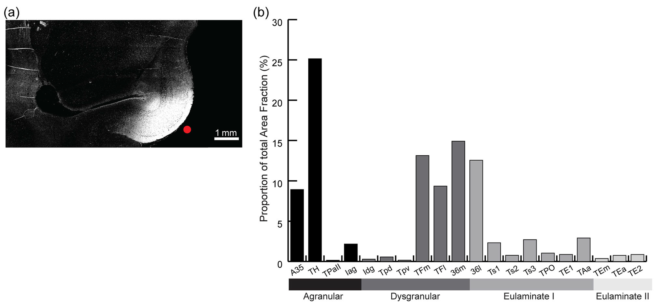
Distribution of terminations in temporal areas from area 28. (a) The injection site of anterograde tracer (tritiated amino acids) in A28 (red dot). (b) Proportion of terminations in distinct architectonic areas as a fraction (%) of all terminations in the temporal lobe in this case.

3.10 |. Relationship of laminar distribution of connections to cortical type

The placement of injections in areas of different cortical type yielded data that allowed us to investigate the relationship of projection neuron density to the type of cortical areas involved. Based on our work and others, cortical connectivity does not only depend on density but is also determined by laminar projection patterns. Cortical layers represent distinct microenvironments and, as emphasized above, systematically vary across different areas. Thus, areas with distinct laminar constituents have distinct cell types. Further, connections arise and terminate in different layers. In the visual cortical system in monkeys (Felleman & Van Essen, 1991), the laminar origin and terminating patterns were related to information flow. We have shown similar systematic variations in laminar pattern of connections in the prefrontal (Barbas & Rempel-Clower, 1997), visual (Hilgetag et al., 2016), and prefrontal to temporal cortices (Rempel-Clower & Barbas, 2000). Thus, we computed the SGI, which is the proportion of projection neurons that emanate from layers II and III for areas in each case. Figure 8 depicts the SGI for areas that included at least 1% of the total number of all labeled neurons in the temporal lobe in each case. As shown in Figure 8a, eulaminate areas with label in a case with Ts2 injection, which is also eulaminate, had an average SGI of ≥0.5, while areas with dysgranular and agranular architecture had an SGI of <0.3.

FIGURE 8.

Supragranular index of temporal areas projecting to different injection sites. The supragranular index (SGI) was calculated as the percent of projection neurons in the supragranular layers in each area projecting to each injection site: (a) Ts2, (b)Ts1/TE1, (c)TE1, (d) A36, and (e) TPro.

In the case with an injection in eulaminate areas Ts1/TE1, and as we saw qualitatively in the coronal sections, the medial, dysgranular part of A36 had a lower SGI, ~0.3, while the lateral, eulaminate, A36 had an index of ~0.6 (not shown). Eulaminate cortices (I and II) with labeled neurons had an SGI greater than 0.5 (Figure 8b).

We saw a similar pattern for the case with an injection in area TE1. Most of the labeled neurons were found in A36, and most of these were found in the lateral, more granular part of A36, which had an SGI of ~0.5. This analysis showed that A36 projected to TE1 through both its supragranular and infragranular layers. All eulaminate I and eulaminate II areas that projected to TE1 had an SGI of >0.6 (Figure 8c).

The laminar distribution analysis of labeled projection neurons directed to rostromedial A36 showed that A28 had a low SGI (<0.2), while TPv, A36 lateral (not shown), Ts1, and TE1 had a high SGI (>0.5), with TE1 having the highest index (Figure 8d).

Most neurons directed to TPro originated from dysgranular areas in the temporal pole (TPro, TPd, TPv) and from the supragranular layers of eulaminate area Ts1, which showed an SGI of ~0.6 (Figure 8e). Lastly, most areas projecting to TPro originated projections largely from supragranular layers, except for A35 and TE1.

We then tested whether differences in the laminar distribution of connections across areas were systematic. Based on our previous work, we have developed a Structural Model for connections, which predicts that the density and laminar connections depend on the type difference (delta) between origin and termination sites (Barbas & Rempel-Clower, 1997). Specifically, the Structural Model predicts that when origin type is greater (more laminated) than termination site type (delta >0), the projection neurons tend to arise from the upper layers (SGI is greater than 50%), while in the reverse direction the SGI is lower than 50%.

We calculated the SGI of the temporal areas that sent projections to each of the injection sites and took the average SGI of areas belonging to each cortical type (Barbas, 1986; Barbas & Rempel-Clower, 1997). We then calculated the cortical type difference between the area of origin and area of termination (the injection site of retrograde tracers) and conducted linear regression analyses between SGI and cortical type difference, as shown in Figure 9 for each case. For injections in both eulaminate (Figure 9a,b,c,f) and dysgranular temporal areas (Figure 9d,e,g), our analyses showed a linear relationship between SGI and type difference. Specifically, we found that the SGI increases as the difference in the cortical type of the linked areas increases. Thus, areas with the most differentiated laminar structure have a higher SGI than those areas that have less delineated layers (dysgranular or agranular cortices). Importantly, it is the structural relationship (delta deviation from 0) between linked areas that determines the relative SGI. This effect is revealed by the quasi-monotonic relationship of connections in Figure 9. The placement of injections in areas of different cortical type yielded data that made it possible to investigate the relational nature of connections. This analysis revealed that the temporal interconnections in the rhesus macaque follow the predictions of the Structural Model (Barbas & Rempel-Clower, 1997), consistent with findings in the primate visual (Hilgetag et al., 2016) and prefrontal (Barbas & Rempel-Clower, 1997) cortices.

FIGURE 9.

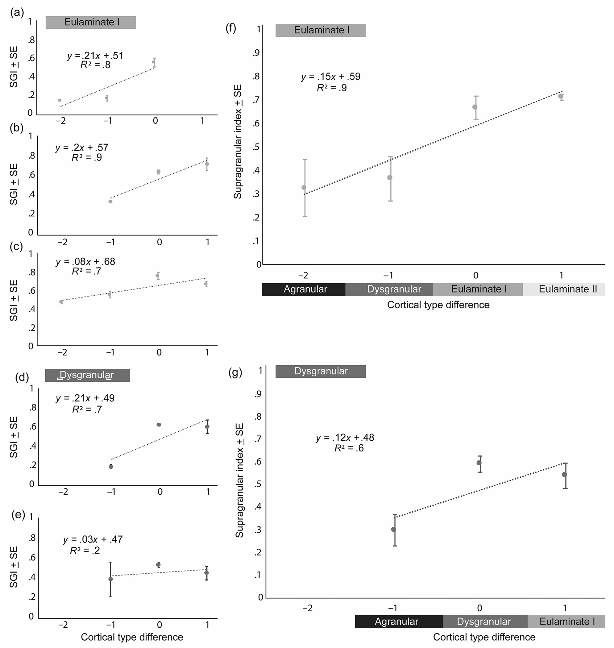
Linear relationship between supragranular index (SGI) and cortical type difference between connected temporal areas. Linear relationships of supragranular index and cortical type difference for individual injection cases in eulaminate areas (a) Ts2, (b)Ts1/TE1, and (c)TE1, and for injections in dysgranular areas (d) A36 and (e)TPro. Linear relationships of average cortical type difference: (f) average supragranular index of temporal areas projecting to eulaminate cortices (average SGI of [a] Ts2, [b]Ts1/TE1, and [c]TE1) and (g) average supragranular index of areas projecting to dysgranular cortices (average SGI of [d] A36 and [e]TPro). The x-axis represents the difference in cortical type between the origin and termination area (origin–termination), where 0 is when connected areas are of the same cortical type, >0 when origin type is greater than termination area type, and <0 is when origin is a lower type than the termination area.

3.11 |. Relationship between connection density and cortical type in the temporal lobe

The density of projection neurons was also strongly linked to cortical type. We found that most of the retrogradely labeled projection neurons originated from areas that were similar in cortical type as the injection site (e.g., eulaminate areas received the densest projections from other eulaminate areas). Similarly, the anterograde injection in agranular A28 showed that it sends projections most densely to other agranular and dysgranular areas.

We then built a matrix based on z-score-normalized density of all connections and then constructed a wire diagram. We color coded connections based on number of cortical “type” boundaries crossed, as shown in Figure 10a. These analyses revealed that similar to the prefrontal and visual cortical systems (Barbas & Rempel-Clower, 1997; Hilgetag et al., 2016), the densest connections between temporal lobe areas occurred between areas with similar cortical types (red) or between areas that differed only by one type (yellow). Connections linking areas that differed by two or more types were sparse (Figure 10a,b, green and blue). Further, we summarized how difference in cortical type predicts laminar pattern, consistent with the Structural Model for laminar connections (Figure 10c). Our data showed that when the area of origin has more differentiated laminar structure (higher cortical type) than the area of termination, the SGI is higher and most neurons originate in the supragranular layers. Thus, eulaminate areas have a higher SGI than agranular/dysgranular areas that have fewer and less delineated layers.

FIGURE 10.

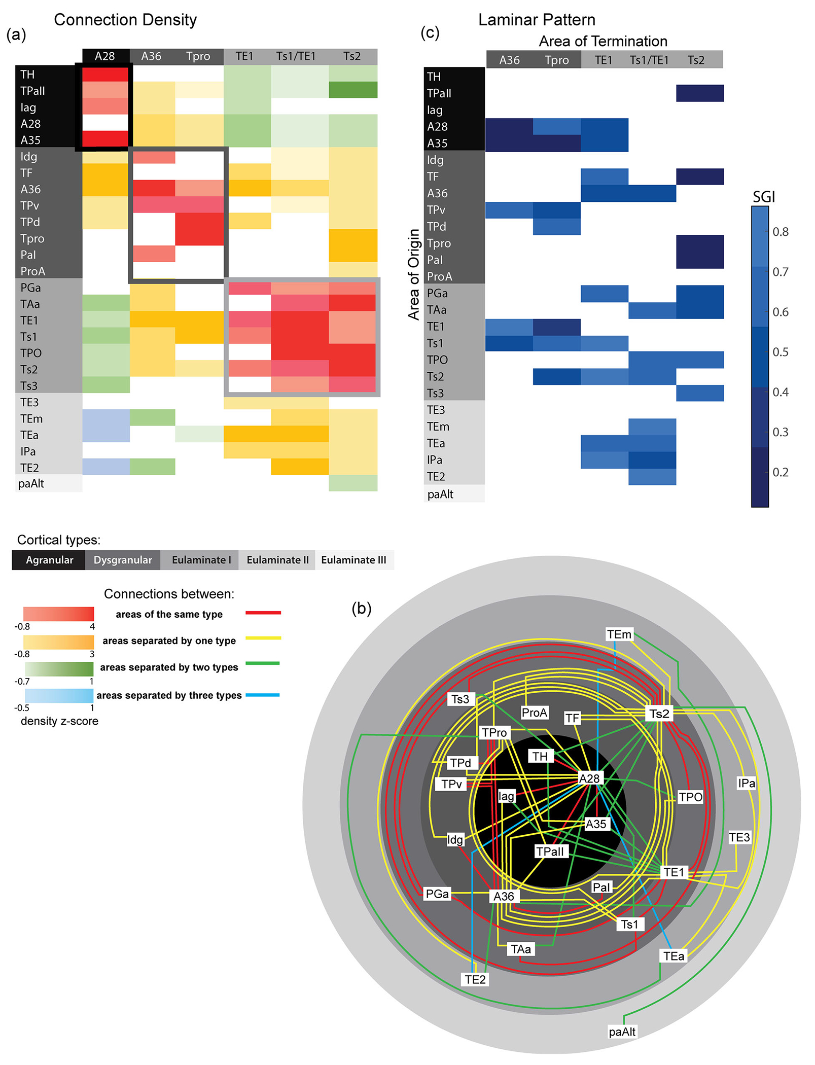
Summary of connections between areas of the temporal lobe by cortical type. (a) A connectional matrix based on the z-scores of normalized densities of all connections. (b) A wired diagram to illustrate connections between areas. Gray shades in panel (b) (also in panels [a] and [c]) represent the level of cortical type from most differentiated (lightest gray, outer rim) to least differentiated (limbic) types (black, center). The matrix and wire diagram connections are color coded based on the cortical type of the areas connected, and the number of cortical “type” boundaries crossed for each connection. The intensity of the color in the matrix represents the z-score value. (c) Summary table showing the scaled supragranular index for each set of projection neurons resulting from retrograde tracer injections (area of termination). When the areas of origin have more differentiated laminar structure (higher cortical type) than its area of termination, the SGI is higher.

3.12 |. Patterns of inhibitory neuronal subpopulations in the EC (A28)

In view of the centrality of A28 in cortical connections within MTL and the hippocampus, we studied its inhibitory microenvironment in the anterior sector, by quantitative analysis of putative inhibitory neurons labeled for the calcium-binding proteins CR, CB, and PV (Figure 11). The advantage of this approach is based on the fact that these neurons show specific laminar distribution in the primate cortex (reviewed in Barbas, 2015), but their specific organization in A28 is not well understood.

FIGURE 11.

The inhibitory microenvironment of anterior entorhinal cortex. (a) Photomicrographs of coronal sections in the entorhinal cortex (EC) stained for Nissl. (b) Photomicrographs of a coronal section through EC stained for calbindin (CB) and counterstained for Nissl: (b1) small inset shows neurons positive for CB at higher magnification below; (b2) inset of medial EC (red outline) stained for CB shows the column at higher magnification below; and (b3) inset from lateral EC column (purple outline) stained for CB shows the column at higher magnification below. (c) Photomicrographs of a coronal section through EC stained for calretinin (CR) and counterstained for Nissl: (c1) small inset shows neurons positive for CR at higher magnification below; (c2) inset of medial EC (red outline) stained for CR shows the column at higher magnification below; and (c3) inset from lateral EC column (purple outline) stained for CR shows the column at higher magnification below. (d) Photomicrographs of a coronal section through EC stained for parvalbumin (PV): (d1) small inset shows neurons positive for PV at higher magnification below; (d2) inset of medial EC (red outline) stained for PV shows the column at higher magnification below; and (d3) Inset from lateral EC column (purple outline) stained for PV shows the column at higher magnification below. amy, amygdala; amts, anterior middle temporal sulcus; E_I, EC intermediate; E_LC, EC lateral caudal; E_LR, EC lateral rostral; E_R, EC rostral; hip, hippocampus; ls, lateral sulcus; rs, rhinal sulcus; sts, superior temporal sulcus.

Our results showed that the highest distribution was noted for CR neurons in all layers combined and in the upper layers (I–III) for both the medial and lateral parts of EC (Figure 12). The density of PV neurons was higher in the lateral than in the medial subdivisions,consistent with previous qualitative data in the human EC (Mikkonen et al., 1997). We found that the density of PV neurons was higher in the deep layers (LD–VI) (Figure 12c) compared to the superficial layers (Figure 12b) in lateral EC; a similar relationship was seen in the medial region of EC but the difference was small. The densities of CB neurons in the medial and lateral EC were comparable across layers (Figure 12a–d), except for layer IIIa (not shown), in which the medial EC had a higher density of CB neurons than the lateral EC, which is consistent with previous findings (Suzuki & Porteros, 2002).

FIGURE 12.

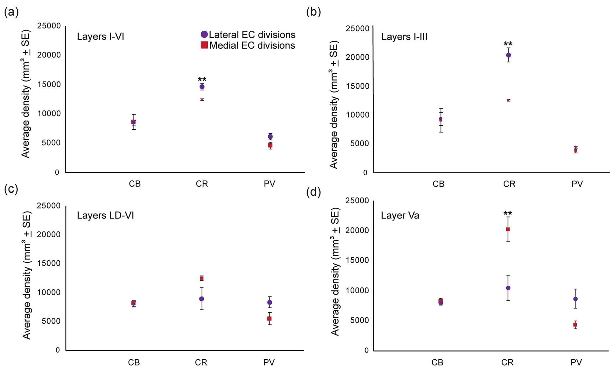
Comparison of the inhibitory microenvironment of the medial and lateral divisions of the anterior entorhinal cortex. (a) Distribution in layers I–VI. (b) Distribution in layers I–III. (c) Distribution from lamina dissecans to VI. (d) Distribution in layer Va. **Statistically significant, p ≤ .05.

4 |. DISCUSSION

Our study of interconnections of temporal lobe areas relied on cases with strategic placement of retrograde tracers in a set of eulaminate areas (e.g., TE1 and Ts2) and dysgranular and agranular (TPro, A36 and A28) areas. These cases yielded label of projection neurons (and in one case terminals) in diverse temporal areas that belong to different cortical types and allowed analysis of connections based on the structural relationship between the injection site and each area with label. Our analyses resulted in two main findings. First, temporal areas received projections largely from other cortical areas of the same or similar cortical type. Second, agranular areas in the temporal lobe primarily projected to eulaminate cortices from their infragranular layers (feedback pattern), while eulaminate areas projected to limbic areas largely from neurons in their supragranular layers (feedforward) in a graded pattern based on the relative difference in laminar structure of the linked areas, as elaborated below.

4.1 |. Distribution of projection neurons in temporal cortices in the context of previous studies

Previous studies have shown that the EC is connected with the PRC and PHC with different strengths (Suzuki & Amaral, 1994b): the perirhinal cortices have dense connections with the rostral two thirds of the EC, whereas the PHC is strongly interconnected with the caudal two thirds of the EC. Moreover, the strength of PRC connections with the EC depends on the mediolateral position of the areas in the PRC (Suzuki & Amaral, 1994b).

Previous work pertaining to the connections of A36 showed that its rostromedial part (A36rm) and rostrolateral division (A36rl) are strongly connected (Lavenex et al., 2004), and our findings align with these observations as well. Our analysis revealed that in a case with a rostromedial A36 injection, the vast majority of labeled neurons originated in rostromedial and rostrolateral divisions of A36 (not shown) and the ventromedial division of TPro (Tpv; Figure 6). Further, in our temporal area TPro case, projection neurons were distributed most densely in auditory association cortices (especially Ts1), in visual area TE, and in dysgranular cortices. Only a few (<1%) of the total projection neurons directed to TPro emanated from A36 and <5% were found in A35. These findings are consistent with previous data, which showed that the temporal polar part of area 36 (36d) has few interconnections with the PRC and PHC, and only the most ventral region of 36d sends projections to A36 (Lavenex et al., 2004).

4.2 |. Relationship of connections to cortical type: The nonlinearity of cascades in and out of hippocampus

Our data confirm and extend previous findings by indicating that for each area studied within the temporal cortex, there is a gradient in the density of projection neurons assessed by quantitative analysis of labeled neurons mapped in the temporal region. In a detailed study, Suzuki and Amaral noted graded density patterns in the interconnections of the EC with PRC and PHC (Suzuki & Amaral, 1994b). In line with the above findings, we found that the intermediate division of the EC included more terminations in the medial part of A36 than in its lateral part. Connections with the PHC also followed a mediolateral gradient, with more terminations in the medial part of TF than its lateral part (Figure 7). Our data extend these findings by relating the density of connections to the broader principle of systematic cortical variation. This principle makes it possible to reduce the high dimensionality of many cortical areas to a few cortical types based on their laminar structure. Our findings revealed that this principle holds even with relatively small differences in overall laminar structure between linked areas, exemplified by the more numerous labeled neurons in the lateral, eulaminate, part of A36 projecting to eulaminate Ts1/TE1, by comparison with fewer projection neurons found in the medial A36, which has a dysgranular architecture. Consistent with this principle are also the more prominent terminations in medial A36 from A28 (Figure 7).

Classical studies have interpreted a sequential pattern of pathways that link multimodal and other high-order association cortices with the hippocampus (e.g., Amaral et al., 1987; Van Hoesen & Pandya, 1975; Van Hoesen et al., 1972). The temporal lobe projections from visual and auditory temporal cortices are reported to be less dense than projections from multimodal cortices (e.g., Mohedano-Moriano et al., 2008). Pathways have also been mapped for the reverse direction from hippocampus to temporal and multisensory areas of the superior temporal sulcus and adjacent temporal high-order sensory association cortices (e.g., Kosel et al., 1982; Munoz & Insausti, 2005). These bidirectional pathways position the EC as the gateway in serial pathways of signals that flow in and out of the hippocampus.

By grouping areas into cortical types, it was possible to show a gradient of connections in each case, whereby areas that have comparable laminar structure are more strongly connected than areas with dissimilar structure. Moreover, the strength of connections of a given area with other areas appears to be monotonic, whereby increasingly bigger differences in laminar structure show progressively sparser connections between linked areas.

Laminar structure is difficult to define concisely, though certain features appear to be critical, namely, the number of identifiable layers and the relative distinction between them (reviewed in Barbas, 2015). In this scheme, the phylogenetically ancient limbic areas have the simplest laminar structure, characterized by lack of layer IV in agranular areas, and the presence of a sparsely populated granular layer IV (dysgranular) areas. In primates, the primary cortices have the most elaborate laminar structure, which is especially prominent in the primary visual cortex.

The vast expanse of cortex between primary and limbic areas is harder to place into cortical types, but several other features help overcome this difficulty. One of these includes density of neurons, which has been used as a proxy for laminar structure, because limbic areas generally have a lower neuron density than the six-layer eulaminate cortices. Neuron density has been used for the connections of visual cortices in several species (e.g., Goulas et al., 2019; Hilgetag et al., 2016), but it is not always the best indicator for cortical type. A more reliable marker is myelination, which is high in primary cortices and low in limbic cortices. For example, the primary motor cortex has a comparatively low neuron density in primates, including the marmoset (Atapour et al., 2019), but it is densely myelinated. Moreover, the pattern of myelin distribution is visible in structural magnetic resonance images in primates by use of the T1/T2 index (Glasser et al., 2016; John et al., 2022; Zhang et al., 2020). Another useful architectonic marker is SMI-32, which labels an intermediate neurofilament protein that is more highly expressed in the cellular layers of eulaminate areas and more sparsely in limbic cortices. SMI-32 is particularly useful because of its high expression in neurons in the deep part of layer III and the upper part of layer V, leaving an unlabeled empty zone in layer IV and making it easier to delineate this layer. This marker is useful for the placement of areas into types, including the specialized primary motor cortex, which has a thin layer IV (Barbas & García-Cabezas, 2015; García-Cabezas & Barbas, 2014).

In recent years, several other cellular and molecular markers and gene expression patterns have been introduced that further define cortical architecture (e.g., Burt et al., 2018; Charvet, 2020; Ding & Van Hoesen, 2010; Ding et al., 2009; Paquola et al., 2020). In combination, several of these markers may provide in the future a cluster of features that can help group areas more accurately into types. Notwithstanding the difficulties of identifying all areas by cortical type, the available markers have made it possible to test the linkage of areas and their strength based on an ordering scheme that takes the above features into account. By this scheme, first used to study the interconnections of prefrontal cortices in rhesus monkeys, the strongest connections occur between areas that have comparable laminar structure (Barbas & Rempel-Clower, 1997), which applies for nearby as well as distantly connected areas (reviewed in Barbas, 2015). Other studies have relied on distance to describe connections (the exponential distance rule, e.g., Markov et al., 2014), which states that the strength of connections declines with distance between linked areas (see also a recent study in marmosets [Theodoni et al., 2021]). For a detailed comparison of models and their power to describe the density and laminar distribution of corticocortical connections, as well as earlier relevant references, see Hilgetag et al. (2016) and a recent study by Aparicio-Rodriguez and Garcia-Cabezas (2023). The detailed analyses showed that distance is not consistently correlated with connection features, but similarity in cortical type successfully predicts the density and laminar distribution of connections (Hilgetag et al., 2016).

4.3 |. Laminar connections are graded by the difference/similarity in type of connected areas

A second issue pertaining to connections is their laminar distribution. Studies of the MTL have shown that projections from the temporal pole, PRC, and PHC to areas outside the MTL originate largely in neurons in the infragranular layers V and VI (Munoz & Insausti, 2005). An infragranular origin has also been reported for projections from EC to PRC and PHC (Suzuki & Amaral, 1994b). Our findings are in general agreement with these findings.

A commonly used analysis for laminar connections is to describe them by the SGI. By this analysis, our findings, in general, show that agranular or dysgranular areas had overall a low SGI, consistent with projection neurons found most densely in the deep layers (V and VI) in limbic areas. The SGI provides an overview of the laminar distribution of connections, but does not capture the fundamental principle, namely, that connections follow a relational rule based on the relative similarity or difference in the structure of the linked areas. Thus, while agranular and dysgranular (limbic) areas project to eulaminate areas from their deep layers, our findings revealed that limbic areas project to each other from both supragranular and infragranular areas, as predicted by the Structural Model (Barbas & Rempel-Clower, 1997). The pattern of projection involving the upper and deep cellular layers of projection neurons, or termination of axons into a columnar pattern in the area of destination, was previously called “lateral” (Felleman & Van Essen, 1991). In the MTL, this relationship is best exemplified in the data of Suzuki and Amaral, who found that the perirhinal and parahippocampal cortices, which are dysgranular, project to EC, which is agranular, predominantly in a feedforward pattern, while EC reciprocates with projections that follow a general feedback pattern (Suzuki & Amaral, 1994b). However, the connections between these limbic areas cannot be easily defined by the broad “feedback–feedforward” dichotomy (see Wellman & Rockland, 1997).

The relationship of connections to the structural type difference/similarity is captured by the Structural Model (Barbas & Rempel-Clower, 1997), which has been substantiated in the connections across several cortical systems, including the visual, and in long-distance connections that link occipital, parietal, and temporal lobes with prefrontal cortices (reviewed in Barbas, 2015). We now found that the pattern also holds for the interconnections within the primate temporal lobe.

4.4 |. The inhibitory microenvironment of EC

The significance of studying the inhibitory microenvironment of EC is based on its position in MTL and connections with the hippocampus. A general finding here is the predominance of CR putative inhibitory neurons, seen both in the upper and deep layers of anterior EC. The predominance of CR neurons in the cortex may be a primate specialization, seen also in anterior cingulate A25 in rhesus monkeys (Joyce et al., 2020) and in humans (Palomero-Gallagher et al., 2008, 2009). In the upper cortical layers, CR neurons in other areas are thought to have a predominantly disinhibitory role, by innervating other inhibitory neurons (e.g., Meskenaite, 1997). The predominance of CR neurons in the upper layers of EC suggests a facilitating role for passage of cortical signals to hippocampus. The specific innervation by CR neurons of nearby neurons is unknown for the deep layers, where they may have a modulatory status by innervating pyramidal neurons, or some may be excitatory.

The density of PV inhibitory neurons, which provide strong perisomatic inhibition of nearby pyramidal neurons, was lower than CR or CB but still substantial. Moreover, PV neuron density was comparable across the layers of the medial subdivisions of the rostral EC, a pattern that differs from other cortical areas in primates, which generally show a higher density of PV neurons in the deep layers (e.g., DeFelipe, 1997; Dombrowski et al., 2001). The comparable distribution of PV neurons across layers in EC suggests a comparable role in influencing pathways that project to hippocampus through the upper layers, as well as in the deep layers that convey signals that project out of the hippocampus for transmission broadly to other cortices.

A caveat of this study is in the limited evidence on the termination of pathways due to the use of mostly retrograde tracers. Such data would make it possible to also study the targeting of efferent local pathways in MTL of distinct inhibitory neurons, as well as excitatory neurons. Previous studies suggest that preferential targeting of corticocortical pathways of inhibitory neurons varies in the cortex. For example, we previously found that ACC A32 innervates a substantial proportion of PV inhibitory neurons in PHC, where the pathway may influence neuronal dynamics and rhythms associated with memory (for discussion, see Bunce & Barbas, 2011). In another study, we found that pathways from ACC A32 innervated a substantial number of CR postsynaptic sites in the upper layers of A28 and A35, suggesting disinhibitory modulation, and facilitated access of signals to hippocampus (Bunce et al., 2013), consistent with the high density of CR neurons in A28 we found here. On the other hand, a pathway from posterior orbitofrontal cortex (pOFC) innervated most densely A36, where its inhibitory postsynaptic targets were dendritic elements labeled for CB, a system associated with increasing signal and reducing noise (Medalla & Barbas, 2009; Wang et al., 2004). Both pathways from A32 and pOFC innervated mostly PV neurons among the three inhibitory classes. Taken together, these studies suggest specificity in targeting by pathways associated with attention from ACC and emotional valuation from pOFC, demonstrating the rich variety of signals that reach MTL.

5 |. CONCLUSION

The temporal lobe is a diverse region, with areas associated with processing of unimodal and multimodal signals, and complex signals associated with memory and emotions. This diversity in function is mediated by a rich architecture that exemplifies the systematic variation of the cortex, which is linked to connections, as studied here. In this context, it is possible to reduce the dimensionality of the complex temporal lobe regions under the general principle of systematic variation. In this scheme, the phylogenetically ancient limbic areas of the temporal lobe reflect flexibility to engage in diverse functions of learning and memory, made possible by the complex inhibitory microenvironments in EC and by cellular and molecular features that allow plasticity (Garcia-Cabezas et al., 2017). On the other hand, the plasticity of limbic areas, as exemplified in MTL, may render these areas vulnerable to several neurodegenerative and psychiatric disorders known to affect this region (reviewed in Braak & Del Tredici, 2015). Importantly, the plasticity–stability of areas is intricately linked to the systematic variation of the cerebral cortex, which also reflects the connections of areas in patterns that likely are laid down in development. Specifically, variation in laminar structure in adulthood may be traced to a variable progenitor zone, which we found to be thinner in human embryos in prospective limbic areas and thicker and enriched in prospective eulaminate areas that show progressive laminar differentiation in adults (Barbas & García-Cabezas, 2016; Garcia-Cabezas et al., 2019). Similar findings were reported recently for the ventral temporal lobe in human embryos, which showed that the EC lacked an outer subventricular zone, which emerged in the adjacent ventral region and expanded in more laterally situated areas (Ding et al., 2022), consistent with progressive elaboration of layers from medial to lateral temporal cortices in primates, as seen here.

DATA AVAILABILITY STATEMENT

The data that support the findings of this study are available from the corresponding author upon reasonable request.

REFERENCES

- Abbie AA (1940). Cortical lamination in the monotremata. Journal of Comparative Neurology, 72, 429–467. [Google Scholar]
- Abbie AA (1942). Cortical lamination in a polyprotodont marsupial, Perameles nasuta. Journal of Comparative Neurology, 76, 509–536. [Google Scholar]
- Aggleton JP, Wright NF, Rosene DL, & Saunders RC (2015). Complementary patterns of direct amygdala and hippocampal projections to the macaque prefrontal cortex. Cerebral Cortex, 25, 4351–4373. 10.1093/cercor/bhv019 [DOI] [PMC free article] [PubMed] [Google Scholar]
- Amaral DG, Insausti R, & Cowan WM (1987). The entorhinal cortex of the monkey: I. Cytoarchitectonic organization. Journal of Comparative Neurology, 264, 326–355. [DOI] [PubMed] [Google Scholar]
- Anderson MC, Bunce JG, & Barbas H (2015). Prefrontal-hippocampal pathways underlying inhibitory control over memory. Neurobiology of Learning and Memory, 134, 145–161. 10.1016/jLnlm.2015.11.008 [DOI] [PMC free article] [PubMed] [Google Scholar]
- Aparicio-Rodriguez G, & Garcia-Cabezas MA (2023). Comparison of the predictive power of two models of cortico-cortical connections in primates: The distance rule model and the structural model. Cerebral Cortex, 33, 8131–8149. 10.1093/cercor/bhad104 [DOI] [PubMed] [Google Scholar]
- Atapour N, Majka P, Wolkowicz IH, Malamanova D, Worthy KH, & Rosa MGP (2019). Neuronal distribution across the cerebral cortex of the marmoset monkey (Callithrix jacchus). Cerebral Cortex, 29(9), 3836–3863. 10.1093/cercor/bhy263 [DOI] [PubMed] [Google Scholar]
- Barbas H. (1986). Pattern in the laminar origin of corticocortical connections. Journal of Comparative Neurology, 252, 415–422. [DOI] [PubMed] [Google Scholar]
- Barbas H. (2015). General cortical and special prefrontal connections: Principles from structure to function. Annual Review of Neuroscience, 38, 269–289. [DOI] [PubMed] [Google Scholar]
- Barbas H, Bunce JG, & Medalla M (2013). Prefrontal pathways that control attention. In Stuss DT & Knight R (Eds.), Principles of frontal lobe functions (2nd ed., pp. 31–48). Oxford University Press. [Google Scholar]
- Barbas H, & García-Cabezas MA (2015). Motor cortex layer 4: Less is more. Trends in Neuroscience, 38(5), 259–261. [DOI] [PMC free article] [PubMed] [Google Scholar]
- Barbas H, & García-Cabezas MA (2016). How the prefrontal executive got its stripes. Current Opinion in Neurobiology, 40, 125–134. 10.1016/j.conb.2016.07.003 [DOI] [PMC free article] [PubMed] [Google Scholar]
- Barbas H, Ghashghaei H, Dombrowski SM, & Rempel-Clower NL (1999). Medial prefrontal cortices are unified by common connections with superior temporal cortices and distinguished by input from memory-related areas in the rhesus monkey. Journal of Comparative Neurology, 410, 343–367. [DOI] [PubMed] [Google Scholar]
- Barbas H, Medalla M, Alade O, Suski J, Zikopoulos B, & Lera P (2005). Relationship of prefrontal connections to inhibitory systems in superior temporal areas in the rhesus monkey. Cerebral Cortex, 15(9), 1356–1370. [DOI] [PubMed] [Google Scholar]
- Barbas H, & Rempel-Clower N (1997). Cortical structure predicts the pattern of corticocortical connections. Cerebral Cortex, 7, 635–646. [DOI] [PubMed] [Google Scholar]
- Blatt GJ, & Rosene DL (1998). Organization of direct hippocampal efferent projections to the cerebral cortex of the rhesus monkey: Projections from CA1, prosubiculum, and subiculum to the temporal lobe. Journal of Comparative Neurology, 392(1), 92–114. [DOI] [PubMed] [Google Scholar]
- Braak H, & Del Tredici K (2015). Neuroanatomy and pathology of sporadic Alzheimer’s disease. Springer. [PubMed] [Google Scholar]
- Bunce JG, & Barbas H (2011). Prefrontal pathways target excitatory and inhibitory systems in memory-related medial temporal cortices. Neuroimage, 55(4), 1461–1474. [DOI] [PMC free article] [PubMed] [Google Scholar]
- Bunce JG, Zikopoulos B, Feinberg M, & Barbas H (2013). Parallel prefrontal pathways reach distinct excitatory and inhibitory systems in memory-related rhinal cortices. Journal of Comparative Neurology, 512(18), 4260–4283. [DOI] [PMC free article] [PubMed] [Google Scholar]
- Burt JB, Demirtas M, Eckner WJ, Navejar NM, Ji JL, Martin WJ, Bernacchia A, Anticevic A, & Murray JD (2018). Hierarchy of transcriptomic specialization across human cortex captured by structural neuroimaging topography. Nature Neuroscience, 9, 1251–1259. 10.1038/s41593-018-0195-0 [DOI] [PMC free article] [PubMed] [Google Scholar]
- Campbell MJ, & Morrison JH (1989). Monoclonal antibody to neurofilament protein (SMI-32) labels a subpopulation of pyramidal neurons in the human and monkey neocortex. Journal of Comparative Neurology, 282, 191–205. [DOI] [PubMed] [Google Scholar]
- Charvet CJ (2020). Closing the gap from transcription to the structural connectome enhances the study of connections in the human brain. Developmental Dynamics, 249, 1047–1061. 10.1002/dvdy.218 [DOI] [PMC free article] [PubMed] [Google Scholar]
- Cowan WM, Gottlieb DI, Hendrickson AE, Price JL, & Woolsey TA (1972). The autoradiographic demonstration of axonal connections in the central nervous system. Brain Research, 37(1), 21–51. 10.1016/0006-8993(72)90344-7 [DOI] [PubMed] [Google Scholar]
- Dart RA (1934). The dual structure of the neopallium: Its history and significance. Journal of Anatomy, 69, 3–19. [PMC free article] [PubMed] [Google Scholar]
- DeFelipe J. (1997). Types of neurons, synaptic connections and chemical characteristics of cells immunoreactive for calbindin-D28K, parvalbumin and calretinin in the neocortex. Journal of Chemical Neuroanatomy, 14(1), 1–19. [DOI] [PubMed] [Google Scholar]
- Desimone R, & Gross CG (1979). Visual areas in the temporal cortex of the macaque. Brain Research, 178, 363–380. [DOI] [PubMed] [Google Scholar]
- Desimone R, & Ungerleider LG (1989). Neural mechanisms of visual processing in monkeys. In Boller F & Grafman J (Eds.), Handbook of neuropsychology (Vol. 2, pp. 267–299). Elsevier Science Publishers B.V. [Google Scholar]
- Ding SL, Royall JJ, Lesnar P, Facer BAC, Smith KA,Wei Y, Brouner K, Dalley RA, Dee N, Dolbeare TA, Ebbert A, Glass IA, Keller NH, Lee F, Lemon TA, Nyhus J, Pendergraft J, Reid R, Sarreal M, … Lein ES (2022). Cellular resolution anatomical and molecular atlases for prenatal human brains. Journal of Comparative Neurology, 530(1), 6–503. 10.1002/cne.25243 [DOI] [PMC free article] [PubMed] [Google Scholar]
- Ding SL, & Van Hoesen GW (2010). Borders, extent, and topography of human perirhinal cortex as revealed using multiple modern neuroanatomical and pathological markers. Human Brain Mapping, 31(9), 1359–1379. 10.1002/hbm.20940 [DOI] [PMC free article] [PubMed] [Google Scholar]
- Ding SL, Van Hoesen GW, Cassell MD, & Poremba A (2009). Parcellation of human temporal polar cortex: A combined analysis of multiple cytoarchitectonic, chemoarchitectonic, and pathological markers. Journal of Comparative Neurology, 514(6), 595–623. [DOI] [PMC free article] [PubMed] [Google Scholar]
- Dombrowski SM, Hilgetag CC, & Barbas H (2001). Quantitative architecture distinguishes prefrontal cortical systems in the rhesus monkey. Cerebral Cortex, 11, 975–988. [DOI] [PubMed] [Google Scholar]
- Felleman DJ, & Van Essen DC (1991). Distributed hierarchical processing in the primate cerebral cortex. Cerebral Cortex, 1, 1–47. [DOI] [PubMed] [Google Scholar]
- Galaburda AM, & Pandya DN (1983). The intrinsic architectonic and connectional organization of the superior temporal region of the rhesus monkey. Journal of Comparative Neurology, 221, 169–184. [DOI] [PubMed] [Google Scholar]
- Gallyas F. (1979). Silver staining of myelin by means of physical development. Neurological Research, 1, 203–209. [DOI] [PubMed] [Google Scholar]
- García-Cabezas MA, & Barbas H (2014). Area 4 has layer IV in adult primates. European Journal of Neuroscience, 39, 1824–1834. [DOI] [PMC free article] [PubMed] [Google Scholar]
- Garcia-Cabezas MA, Hacker JL, & Zikopoulos B (2022). Homology of neocortical areas in rats and primates based on cortical type analysis: An update of the Hypothesis on the Dual Origin of the Neocortex. Brain Structure & Function, 228, 1069–1093. 10.1007/s00429-022-02548-0 [DOI] [PMC free article] [PubMed] [Google Scholar]
- García-Cabezas MA, John YJ, Barbas H, & Zikopoulos B (2016). Distinction of neurons, glia and endothelial cells in the cerebral cortex: An algorithm based on cytological features. Frontiers in Neuroanatomy, 10, Article 107. 10.3389/fnana.2016.00107 [DOI] [PMC free article] [PubMed] [Google Scholar]
- Garcia-Cabezas MA, Joyce MP, John Y, Zikopoulos B, & Barbas H (2017). Mirror trends of plasticity and stability indicators in primate prefrontal cortex. European Journal of Neuroscience, 46(8), 2392–2405. [DOI] [PMC free article] [PubMed] [Google Scholar]
- Garcia-Cabezas MA, Zikopoulos B, & Barbas H (2019). The Structural Model: A theory linking connections, plasticity, pathology, development and evolution of the cerebral cortex. Brain Structure & Function, 224(3), 985–1008. 10.1007/s00429-019-01841-9 [DOI] [PMC free article] [PubMed] [Google Scholar]
- Glasser MF, Coalson TS, Robinson EC, Hacker CD, Harwell J, Yacoub E, Ugurbil K, Andersson J, Beckmann CF, Jenkinson M, Smith SM, & Van Essen DC (2016). A multi-modal parcellation of human cerebral cortex. Nature, 536(7615), 171–178. 10.1038/nature18933 [DOI] [PMC free article] [PubMed] [Google Scholar]
- Goulas A, Majka P, Rosa MGP, & Hilgetag CC (2019). A blueprint of mammalian cortical connectomes. PLoS Biology, 17(3), Article e2005346. 10.1371/journal.pbio.2005346 [DOI] [PMC free article] [PubMed] [Google Scholar]
- Gross CG, Desimone R, Albright TD, & Schwartz EL (1984). Inferior temporal cortex as a visual integration area. In Reinoso-Suarez F & Ajmone-Marsan C (Eds.), Cortical integration (pp. 291–315). Raven Press. [Google Scholar]
- Gundersen HJ (1986). Stereology of arbitrary particles. A review of unbiased number and size estimators and the presentation of some new ones, in memory of William R. Thompson. Journal of Microscopy, 143(Pt 1), 3–45. [PubMed] [Google Scholar]
- Hilgetag CC, Medalla M, Beul S, & Barbas H (2016). The primate connectome in context: Principles of connections of the cortical visual system. Neuroimage, 134, 685–702. 10.1016/j.neuroimage.2016.04.017 [DOI] [PMC free article] [PubMed] [Google Scholar]
- Hoistad M, & Barbas H (2008). Sequence of information processing for emotions through pathways linking temporal and insular cortices with the amygdala. Neuroimage, 40(3), 1016–1033. [DOI] [PMC free article] [PubMed] [Google Scholar]
- Howard CV, & Reed MG (1998). Unbiased stereology: Three-dimensional measurement in microscopy (Vol. 1). BIOS Scientific Publishers Limited. [Google Scholar]
- Jiao Y, Sun Z, Lee T, Fusco FR, Kimble TD, Meade CA, Cuthbertson S, & Reiner A (1999). A simple and sensitive antigen retrieval method for free-floating and slide-mounted tissue sections. Journal of Neuroscience Methods, 93(2), 149–162. [DOI] [PubMed] [Google Scholar]
- John YJ, Zikopoulos B, Garcia-Cabezas MA, & Barbas H (2022). The cortical spectrum: A robust structural continuum in primate cerebral cortex revealed by histological staining and magnetic resonance imaging. Frontiers in Neuroanatomy, 16, Article 897237. 10.3389/fnana.2022.897237 [DOI] [PMC free article] [PubMed] [Google Scholar]
- Joyce MKP, Garcia-Cabezas MA, John YJ, & Barbas H (2020). Serial prefrontal pathways are positioned to balance cognition and emotion in primates. Journal of Neuroscience, 40(43), 8306–8328. 10.1523/JNEUROSCI.0860-20.2020 [DOI] [PMC free article] [PubMed] [Google Scholar]
- Kosel KC, Van Hoesen GW, & Rosene DL (1982). Non-hippocampal cortical projections from the entorhinal cortex in the rat and rhesus monkey. Brain Research, 244(2), 201–213. [DOI] [PubMed] [Google Scholar]
- Lavenex P, & Amaral DG (2000). Hippocampal-neocortical interaction: A hierarchy of associativity. Hippocampus, 10(4), 420–430. [DOI] [PubMed] [Google Scholar]
- Lavenex P, Suzuki WA, & Amaral DG (2002). Perirhinal and parahippocampal cortices of the macaque monkey: Projections to the neocortex. Journal of Comparative Neurology, 447(4), 394–420. [DOI] [PubMed] [Google Scholar]
- Lavenex P, Suzuki WA, & Amaral DG (2004). Perirhinal and parahippocampal cortices of the macaque monkey: Intrinsic projections and interconnections. Journal of Comparative Neurology, 472(3), 371–394. [DOI] [PubMed] [Google Scholar]
- Liu X, Bautista J, Liu E, & Zikopoulos B (2020). Imbalance of laminar-specific excitatory and inhibitory circuits of the orbito frontal cortex in autism. Research Square, 10.21203/rs.3.rs-29733/v1 [DOI] [PMC free article] [PubMed] [Google Scholar]
- Markov NT, Vezoli J, Chameau P, Falchier A, Quilodran R, Huissoud C, Lamy C, Misery P, Giroud P, Ullman S, Barone P, Dehay C, Knoblauch K, & Kennedy H (2014). Anatomy of hierarchy: Feedforward and feedback pathways in macaque visual cortex. Journal of Comparative Neurology, 522(1), 225–259. 10.1002/cne.23458 [DOI] [PMC free article] [PubMed] [Google Scholar]
- Medalla M, & Barbas H (2009). Synapses with inhibitory neurons differentiate anterior cingulate from dorsolateral prefrontal pathways associated with cognitive control. Neuron, 61(4), 609–620. [DOI] [PMC free article] [PubMed] [Google Scholar]
- Medalla M, & Barbas H (2014). Specialized prefrontal “auditory fields”: Organization of primate prefrontal-temporal pathways. Frontiers in Neuroscience, 8, Article 77. 10.3389/fnins.2014.00077 [DOI] [PMC free article] [PubMed] [Google Scholar]
- Meskenaite V. (1997). Calretinin-immunoreactive local circuit neurons in area 17 of the cynomolgus monkey, Macaca fascicularis. Journal of Comparative Neurology, 379(1), 113–132. [PubMed] [Google Scholar]
- Mikkonen M, Soininen H, & Pitkanen A (1997). Distribution of parvalbumin-, calretinin-, and calbindin-D28k- immunoreactive neurons and fibers in the human entorhinal cortex. Journal of Comparative Neurology, 388, 64–88. [PubMed] [Google Scholar]
- Mohedano-Moriano A, Martinez-Marcos A, Pro-Sistiaga P, Blaizot X, Arroyo-Jimenez MM, Marcos P, Artacho-Pérula E, & Insausti R (2008). Convergence of unimodal and polymodal sensory input to the entorhinal cortex in the fascicularis monkey. Neuroscience, 151(1), 255–271. [DOI] [PubMed] [Google Scholar]
- Munoz M, & Insausti R (2005). Cortical efferents of the entorhinal cortex and the adjacent parahippocampal region in the monkey (Macaca fascicularis). European Journal of Neuroscience, 22(6), 1368–1388. [DOI] [PubMed] [Google Scholar]
- Palomero-Gallagher N, Mohlberg H, Zilles K, &Vogt B. (2008). Cytology and receptor architecture of human anterior cingulate cortex. Journal of Comparative Neurology, 508(6), 906–926. 10.1002/cne.21684 [DOI] [PMC free article] [PubMed] [Google Scholar]
- Palomero-Gallagher N, Vogt BA, Schleicher A, Mayberg HS, & Zilles K (2009). Receptor architecture of human cingulate cortex: Evaluation of the four-region neurobiological model. Human Brain Mapping, 30(8), 2336–2355. 10.1002/hbm.20667 [DOI] [PMC free article] [PubMed] [Google Scholar]
- Pandya DN, & Sanides F. (1973). Architectonic parcellation of the temporal operculum in rhesus monkey and its projection pattern. Zeitschrift für Anatomie und Entwicklungsgeschichte, 139, 127–161. [DOI] [PubMed] [Google Scholar]
- Paquola C, Seidlitz J, Benkarim O, Royer J, Klimes P, Bethlehem RAI, Larivière S, Vos de Wael R, Rodríguez-Cruces R, Hall JA, Frauscher B, Smallwood J, & Bernhardt BC (2020). A multi-scale cortical wiring space links cellular architecture and functional dynamics in the human brain. PLoS Biology, 18(11), Article e3000979. 10.1371/journal.pbio.3000979 [DOI] [PMC free article] [PubMed] [Google Scholar]
- Rasband WS (1997–2014). ImageJ. http://imagej.nih.gov/ij/ [Google Scholar]
- Reiner A, Veenman CL, Medina L, Jiao Y, Del Mar N, & Honig MG (2000). Pathway tracing using biotinylated dextran amines. Journal of Neuroscience Methods, 103(1), 23–37. [DOI] [PubMed] [Google Scholar]
- Rempel-Clower NL, & Barbas H (2000). The laminar pattern of connections between prefrontal and anterior temporal cortices in the rhesus monkey is related to cortical structure and function. Cerebral Cortex, 10(9), 851–865. [DOI] [PubMed] [Google Scholar]
- Richmond FJR,Gladdy R,Creasy JL, Ditamura S,Smits E,&Thomson DB. (1994). Efficacy of seven retrograde tracers, compared in multiplelabelling studies of feline motoneurones. Journal of Neuroscience Methods, 53, 35–46. [DOI] [PubMed] [Google Scholar]
- Rosene DL, Roy NJ, & Davis BJ (1986). A cryoprotection method that facilitates cutting frozen sections of whole monkey brains from histological and histochemical processing without freezing artifact. Journal of Histochemistry and Cytochemistry, 34, 1301–1315. [DOI] [PubMed] [Google Scholar]
- Rosene DL, & Van Hoesen GW (1977). Hippocampal efferents reach widespread areas of cerebral cortex and amygdala in the rhesus monkey. Science, 198, 315–317. [DOI] [PubMed] [Google Scholar]
- Rosene DL, &Van Hoesen GW. (1987). The hippocampal formation of the primate brain. A review of some comparative aspects of cytoarchitecture and connections. In Jones EG & Peters A (Eds.), Cerebral cortex (Vol. 6, pp. 345–455). Plenum Publishing Corporation. [Google Scholar]
- Sakai K, & Miyashita Y (1993). Memory and imagery in the temporal lobe. Current Opinion in Neurobiology, 3(2), 166–170. 10.1016/0959-4388(93)90205-d [DOI] [PubMed] [Google Scholar]
- Saleem KS, Price JL, & Hashikawa T (2007). Cytoarchitectonic and chemoarchitectonic subdivisions of the perirhinal and parahippocampal cortices in macaque monkeys. Journal of Comparative Neurology, 500(6), 973–1006. [DOI] [PubMed] [Google Scholar]
- Sanides F (1969). Comparative architectonics of the neocortex of mammals and their evolutionary interpretation. Annals of the New York Academy of Sciences, 167, 404–423. [Google Scholar]
- Saunders RC, & Rosene DL (1988). A comparison of the efferents of the amygdala and the hippocampal formation in the rhesus monkey: I. Convergence in the entorhinal, prorhinal, and perirhinal cortices. Journal of Comparative Neurology, 271, 153–184. [DOI] [PubMed] [Google Scholar]
- Seltzer B, & Pandya DN (1978). Afferent cortical connections and architectonics of the superior temporal sulcus and surrounding cortex in the rhesus monkey. Brain Research, 149, 1–24. [DOI] [PubMed] [Google Scholar]
- Squire LR, Stark CE, & Clark RE (2004). The medial temporal lobe. Annual Review of Neuroscience, 27, 279–306. [DOI] [PubMed] [Google Scholar]
- Suzuki WA, & Amaral DG (1994a). Perirhinal and parahippocampal cortices of the macaque monkey: Cortical afferents. Journal of Comparative Neurology, 350, 497–533. [DOI] [PubMed] [Google Scholar]
- Suzuki WA, & Amaral DG (1994b). Topographic organization of the reciprocal connections between the monkey entorhinal cortex and the perirhinal and parahippocampal cortices. Journal of Neuroscience, 14, 1856–1877. [DOI] [PMC free article] [PubMed] [Google Scholar]
- Suzuki WA, & Amaral DG (2003). Perirhinal and parahippocampal cortices of the macaque monkey: Cytoarchitectonic and chemoarchitectonic organization. Journal of Comparative Neurology, 463(1), 67–91. [DOI] [PubMed] [Google Scholar]
- Suzuki WA, & Eichenbaum H (2000). The neurophysiology of memory. Annals of the New York Academy of Sciences, 911, 175–191. [DOI] [PubMed] [Google Scholar]
- Suzuki WA, & Porteros A (2002). Distribution of calbindin D-28k in the entorhinal, perirhinal, and parahippocampal cortices of the macaque monkey. Journal of Comparative Neurology, 451(4), 392–412. [DOI] [PubMed] [Google Scholar]
- Theodoni P, Majka P, Reser DH, Wojcik DK, Rosa MGP, & Wang XJ (2021). Structural attributes and principles of the neocortical connectome in the marmoset monkey. Cerebral Cortex, 32(1), 15–28. 10.1093/cercor/bhab191 [DOI] [PMC free article] [PubMed] [Google Scholar]
- Van Hoesen GW, & Pandya DN(1975). Some connections of the entorhinal (area 28) and perirhinal (area 35) cortices of the rhesus monkey. III. Efferent connections. Brain Research, 95(1), 39–59. [DOI] [PubMed] [Google Scholar]
- Van Hoesen GW, Pandya DN, & Butters N (1972). Cortical afferents to the entorhinal cortex of the rhesus monkey. Science, 175, 1471–1473. [DOI] [PubMed] [Google Scholar]
- Veenman CL, Reiner A, & Honig MG (1992). Biotinylated dextran amine as an anterograde tracer for single- and double-labeling studies. Journal of Neuroscience Methods, 41(3), 239–254. [DOI] [PubMed] [Google Scholar]
- von Economo C. (1927/2009). Cellular structure of the human cerebral cortex (Lazaros CT, Trans.). Karger. [Google Scholar]
- Wang XJ, Tegner J, Constantinidis C, &Goldman-Rakic PS. (2004). Division of labor among distinct subtypes of inhibitory neurons in a cortical microcircuit of working memory. Proceedings of the National Academy of Sciences of the United States of America, 101(5), 1368–1373. [DOI] [PMC free article] [PubMed] [Google Scholar]
- Wellman BJ, & Rockland KS (1997). Divergent cortical connections to entorhinal cortex from area TF in the macaque. Journal of Comparative Neurology, 389, 361–376. [PubMed] [Google Scholar]
- Xiao D, Zikopoulos B, & Barbas H (2009). Laminar and modular organization of prefrontal projections to multiple thalamic nuclei. Neuroscience, 161(4), 1067–1081. [DOI] [PMC free article] [PubMed] [Google Scholar]
- Zhang J, Scholtens LH, Wei Y, van den Heuvel MP, Chanes L, & Barrett LF (2020). Topography impacts topology: Anatomically central areas exhibit a “high-level connector” profile in the human cortex. Cerebral Cortex, 30(3), 1357–1365. 10.1093/cercor/bhz171 [DOI] [PMC free article] [PubMed] [Google Scholar]
- Zikopoulos B, John YJ, García-Cabezas MA, Bunce JG, & Barbas H (2016). The intercalated nuclear complex of the primate amygdala. Neuroscience, 330, 267–290. 10.1016/j.neuroscience.2016.05.052 [DOI] [PMC free article] [PubMed] [Google Scholar]
Associated Data
This section collects any data citations, data availability statements, or supplementary materials included in this article.