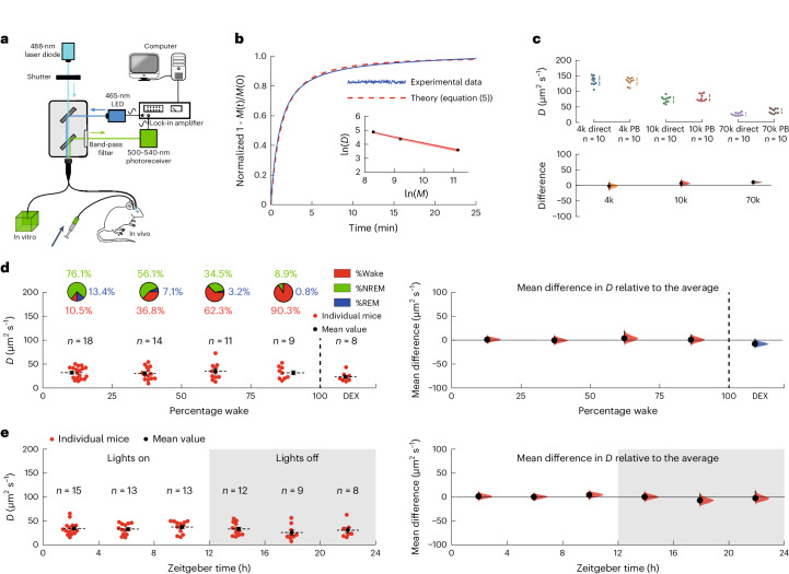
Fig. 1. Changes in local diffusion with vigilance states.
a, The experimental setup. Light from a 488-nm laser diode was passed through a 200-μm optical fiber into either an agarose gel brain phantom in vitro or the frontal cortex of a mouse in vivo. For the in vitro experiments, the agarose gel contained 4 kDa FITC-dextran while, for the in vivo experiments, the brain had been injected with 4 kDa FITC-dextran some hours earlier. b, A typical recording of photobleaching in an agarose gel brain phantom, fitted by least-squares to equation (5), to give (for this example) a value of D = 136 μm2 s−1. The inset shows that the diffusion coefficient follows a power law, with D ∝ M−0.44. The red shading in the inset shows the s.e.m. c, A comparison between the diffusion coefficients determined directly (direct) (Methods and Extended Data Fig. 3) and those determined using the photobleaching method (PB) was not significantly different (two-way ANOVA P = 0.10). Top, the individual data points. Bottom, the differences in the diffusion coefficients determined using the two methods. The agreement between the methods was excellent at 4 kDa FITC-dextran and this was used for the in vivo measurements. d, Left, the diffusion coefficients of 4 kDa FITC-dextran as a function of the percentage of wake (state) during the hour the diffusion coefficient was being measured (the distribution of vigilance states is shown in the pie charts above). Each point represents the average of typically four measurements for an individual mouse and the number of mice, n, is shown above. The last group of data on the right-hand side were recorded during dexmedetomidine (DEX) sedation. Right, the mean differences relative to the average diffusion coefficient across all vigilance states. A one-way ANOVA gave F(4,55) = 0.90; P = 0.47. (A difference of ~35% in D would have been detected.) e, Left, the diffusion coefficients as a function of zeitgeber time. Right, the mean differences relative to the average diffusion coefficient recorded over the circadian cycle. A one-way ANOVA gave F(5,64) = 0.88; P = 0.50. In c–e, the vertical solid lines show the 95% confidence intervals; the shaded areas show the distributions of likelihood. In d and e, the horizontal solid and dashed lines show the s.e.m. and the mean, respectively.

