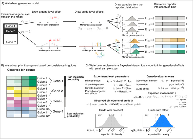
Figure 2: A statistical model for CRISPR FACS screen data.

A) Overview of the generative model. First, the gene level perturbation effect is assessed as either having a no effect (top row) or having an effect (bottom row) on the marker gene and the effect size established as μ₁. For genes with an effect on the marker, the individual gRNA effect sizes are chosen centered around this gene effect. Each gRNA is assumed to shift the expression of the marker gene to center on the gRNA’s effect size. Finally, each marker is discretized into four FACS bins with the counts in each bin reflecting the amount that the marker distribution was shifted. B) Multiple gRNAs that have consistent effects on a given gene increase the probability that perturbation of that gene affects the level of the marker. In this example, gRNAs 1–3 target Gene 1 and show a consistent up regulation of the marker, thus, Gene 1 has the highest posterior inclusion probability. gRNAs 4–6 have more noise and less overall up regulation, so Gene 2 shows a slightly lower posterior inclusion probability than Gene 1. C) Waterbear implements a Bayesian hierarchical model to infer gene-level effects with small sample sizes by sharing parameters within genes and across the experiment. Additionally, Waterbear improves inference by modeling the unobserved FACS distribution (bottom row). When there is no shift, the guide distribution is modeled to look like a control guide (bottom left). When there is an effect, the bin proportion and thus bin counts are shifted (bottom right).