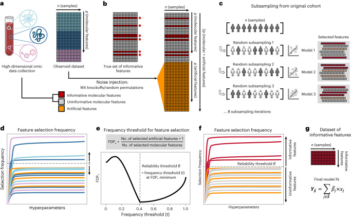
Fig. 1. Overview of the Stabl algorithm.

a, An original dataset of size n × p is obtained from measurement of p molecular features in each of n samples. b, Among the observed features, some are informative (related to the outcome, red), and others are uninformative (unrelated to the outcome, gray). p artificial features (orange), all uninformative by construction, are injected into the original dataset to obtain a new dataset of size n × 2p. Artificial features are constructed using MX knockoffs or random permutations. c, B subsample iterations are performed from the original cohort of size n. At each iteration k, SRM models varying in their regularization parameter(s) λ are fitted on the subsample, resulting in a different set of selected features for each iteration. d, For a given λ, B sets of selected features are generated in total. The proportion of sets in which feature i is present defines the feature selection frequency f_i(λ). Plotting f_i(λ) against 1/λ yields a stability path graph. Features whose maximum frequency is above a frequency threshold (t) are selected in the final model. e, Stabl uses the reliability threshold (θ), obtained by computing the minimum value of the FDP₊ (Methods). f,g, The feature set with a selection frequency larger than θ (that is, reliable features) is included in a final predictive model.