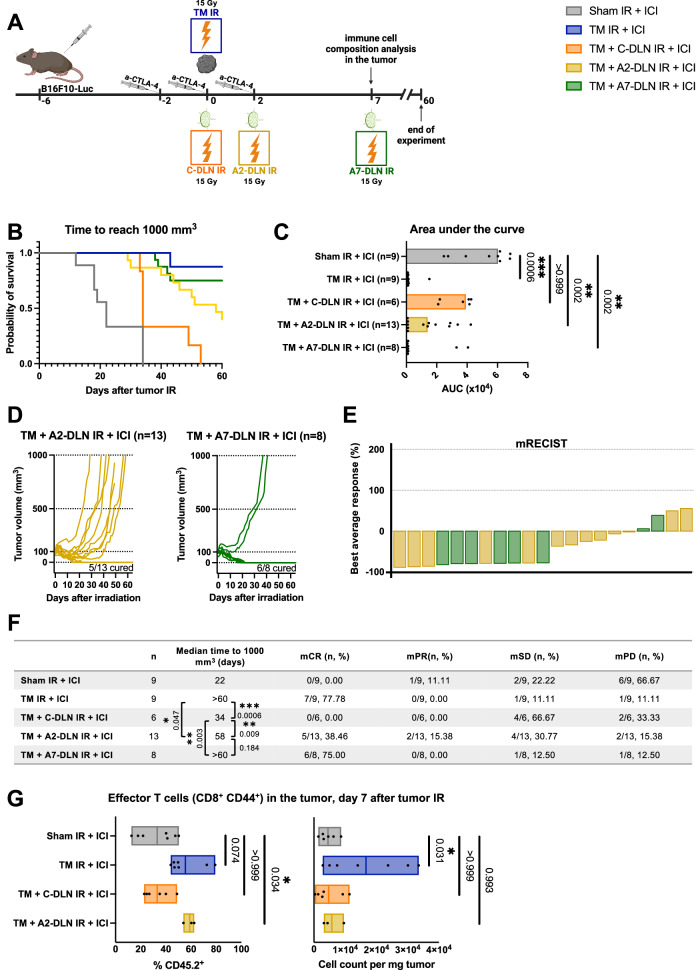
Fig. 4. Delayed (adjuvant) draining lymph node irradiation preserves the efficacy of radioimmunotherapy.

A B16F10-Luc tumor-bearing mice received α-CTLA-4 and tumor IR, with or without DLN IR at different timepoints. All groups received α-CTLA-4. “Sham IR + ICI” group (gray) was sham-irradiated, “TM IR + ICI” group (blue) received tumor IR, “TM + C-DLN IR + ICI” group (orange) received DLN IR concomitantly to the tumor IR, “TM + A2-DLN IR + ICI” (yellow) and “TM + A7-DLN IR + ICI” (green) received DLN IR delayed by 2 and 7 days, respectively. Tumor growth was followed over 60 days. Immune cell composition was analyzed on day 7 after tumor IR. B–F Treatment response represented by the Kaplan–Meier survival analysis (B and F), area under the curve (AUC) analysis (C), individual tumor growth curves (D) and a waterfall plot derived from the mRECIST analysis (E). Time to reach 1000 mm³ was used as the endpoint for Kaplan–Meier analysis. Each dot in C, each line in D and each bar in E represents an individual mouse. Bar width in C represents the median value of the corresponding group. Parameters derived from the mRECIST analysis in E and F are described in the Methods section. mCR complete response, mPR partial response, mSD stable disease, mPD progressive disease. Number of mice in each group is indicated in F. G Tumor-infiltrating effector T cells on day 7 after tumor IR. Left: Effector T cells as a percentage of CD45⁺ cells, right: cell count per mg tumor. Gating strategy is shown in Supplementary Fig. 1A. Each dot represents an individual mouse. Floating bars span from the minimal to the maximal value of each group. Line indicates the mean. n ≥ 3 mice per group (exact numbers provided in Source Data file). Data were tested for normality using the Shapiro–Wilk test. For data following a normal distribution, treatment groups were compared using the one-way ANOVA with Holm–Sidak’s multiple comparisons test (G, right). For non-normally distributed data, the comparisons were performed using the Kruskal–Wallis test with Dunn’s multiple comparisons test (C and G, left). Logrank test (Mantel–Cox) was used to compare the survival curves; corresponding p values are displayed in F. All p values are displayed, with *, ** and *** indicating p < 0.05, p < 0.01 and p < 0.001, respectively. Source data are provided as a Source Data file. Figure A, created with BioRender.com, released under a Creative Commons Attribution-NonCommercial-NoDerivs 4.0 International license.