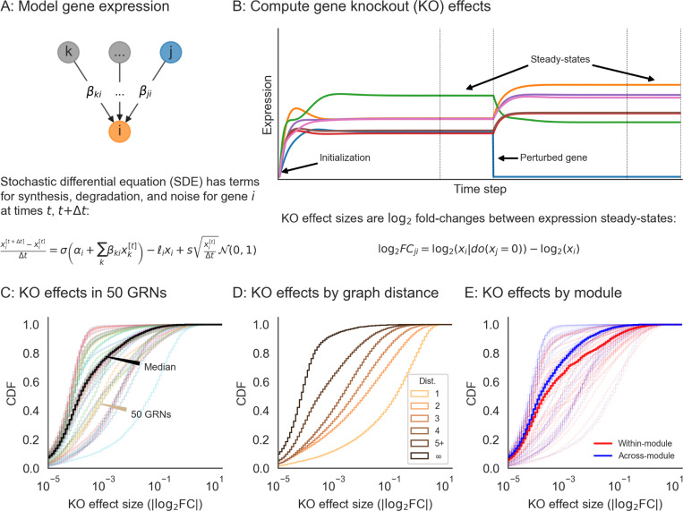
Figure 3: Perturbations and their effects within networks.

(A) Overview of gene expression model and its parameters. Here, $\sigma$ is the logistic sigmoid $\sigma (x)=1/\left(1+e^{-x}\right)$. (B) Example forward simulation of the dynamical systems model. Trace lines show genes, whose expression values are initialized at zero. The system eventually reaches a steady-state, and is then subject to perturbation (knockout of gene $j$, i.e. holding $x_j=0$). Further forward simulation leads to a new steady-state, from which we can compute perturbation effects (log₂ FC for other genes $i$). (C) Distribution of knockout (KO) effects (i.e., log₂ fold-changes in expression $x_i$ of a focal gene $i$) in 50 example GRNs, along with the median distribution (black line). (D) KO effects as a function of network distance between two genes, and (E) within and across modules given by the generating algorithm. Note that the solid lines in (D) and (E) are the median distributions over the 50 example GRNs, split respectively by distances and modules.